Case study 2: Yam and sorghum landscape connectivity in Sub-Saharan Africa

The scope of this vignette is to show how you can implement the crop landscape connectivity throughout a continent or region using MAPSPAM data in the geohabnet package.

Download required packages

Download required packages and set the color palettes

library(terra)

## Warning: package 'terra' was built under R version 4.5.2

## terra 1.9.27

library(geodata)
library(geohabnet)
library(viridisLite)

## Warning: package 'viridisLite' was built under R version 4.5.2

library(rworldmap)

## Loading required package: sp

## ### Welcome to rworldmap ###

## For a short introduction type :   vignette('rworldmap')

data("countriesLow")

vir.pal<-viridisLite::viridis(n=100, option = "inferno", direction = -1, begin = 0.05, end = 0.95)
paldif <- viridisLite::viridis(80, option = "cividis", direction = -1, alpha = 1)

Set the geographical extent

If you want to focus on a specific area such as a country, region or continent, you can set the target extent and crop your dataset.

#----------- Africa -------------------
afr_ext <- ext(-26, 58, -35, 26)

#----------- West Africa -------------------
westafr_ext <- ext(-18, 14, 3, 17)

Download the crop havested area files and plot the cropland density map

You can use the crop_spam() function in the geodata package to download cropland data into MAPSPAM. Using this function, global map file data is extracted from “SPAM 2010 v2.0 Global Data (Updated 2020-07-15)”, and sub-Saharan map file data is extracted from “SPAM 2017 v2.1 Sub-Saharan Africa (Updated 2020-12-21)”. A new global map file has recently been made available via “SPAM 2020 v1.0 Global data (Updated 2024-04-16)”, but is not yet taken into account by the function.You must download the raster file to your computer before using it in r, or upload it directly online. Note: MAPSPAM pixel values are expressed in hectares, so we divide them by 10,000 to convert them into square kilometers, to provide a uniform measure for comparing landscape across different regions.

Here we use the example of sorghum in the sub-African region and yam in West Africa.

# sorghum
sorghumland.density <- geodata::crop_spam(crop = "sorghum", "harv_area", path = tempdir(), africa = FALSE)
sorghumland.density <- sorghumland.density$sorghum_harv_area_all/10000

plot(sorghumland.density, col = vir.pal, main = "sorghumland density")
plot(countriesLow, add=TRUE, border = "grey25", lwd = 0.5)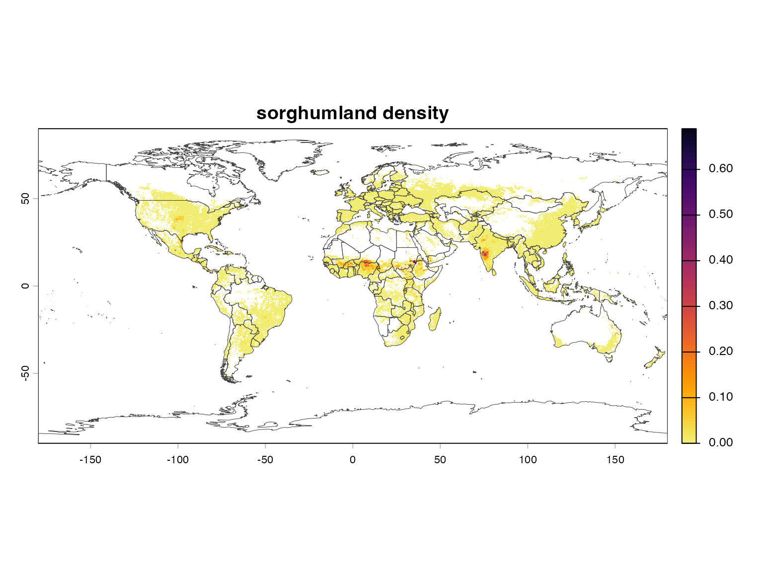

# yams
yamsland.density <- geodata::crop_spam(crop = "yams", "harv_area", path = tempdir(), africa = FALSE)
yamsland.density <- yamsland.density$yams_harv_area_all/10000
yamsland.density <- crop(yamsland.density, westafr_ext)

plot(yamsland.density, col = vir.pal, main = "yamsland density")
plot(countriesLow, add=TRUE, border = "grey25")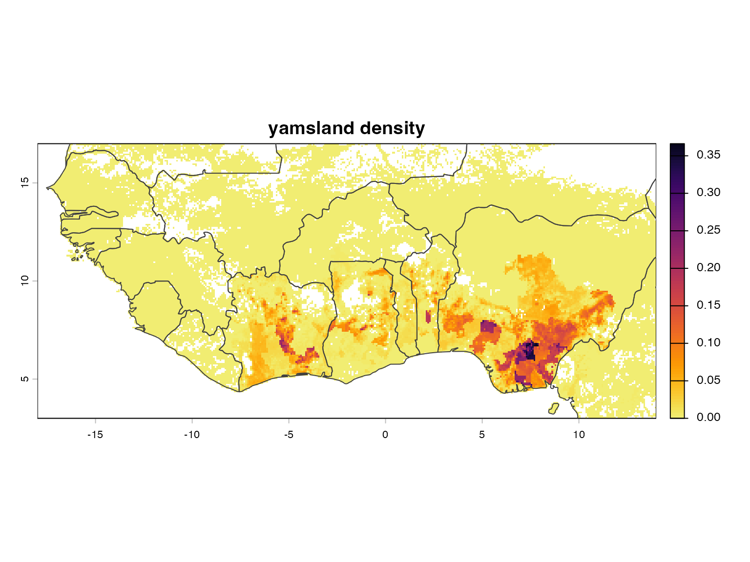

Cropland connectivity

You can use the sean() or msean() functions in the geohabnet package to perform sensitivity analysis of cropland connectivity. To perform this analysis, you can choose to use the default parameter values available in msean(), or you can customize the parameter values according to your understanding of the analysis and the cropping system you are working on.

Sorghum landscape connectivity in the sub-African region

In the fist analysis, we are using the default parameters values in msean(). The four default network metrics are betweeness centrality (weighted 50%), node strength (weighted 15%), Sum of nearest neighbors (weighted 15%), and eigenvector centrality (weighted 20%). The link_threshold and hd_threshold values equal to 0.00001 and 0.0025 respectively are well explained in Xing et al. (2020).

In the second analysis, we changed the betweeness centrality metric within the four network metrics with closeness centrality

# First analysis: using the default parameter values

sorghumland.connectivity<-msean(sorghumland.density,
                                         agg_methods = c("mean"), dist_method = "geodesic",
                                         link_threshold =  0.00001, hd_threshold = 0.0025,
                                         res = 12, global = FALSE, geoscale = c(-26, 58, -35, 26))

## Warning: package 'future' was built under R version 4.5.2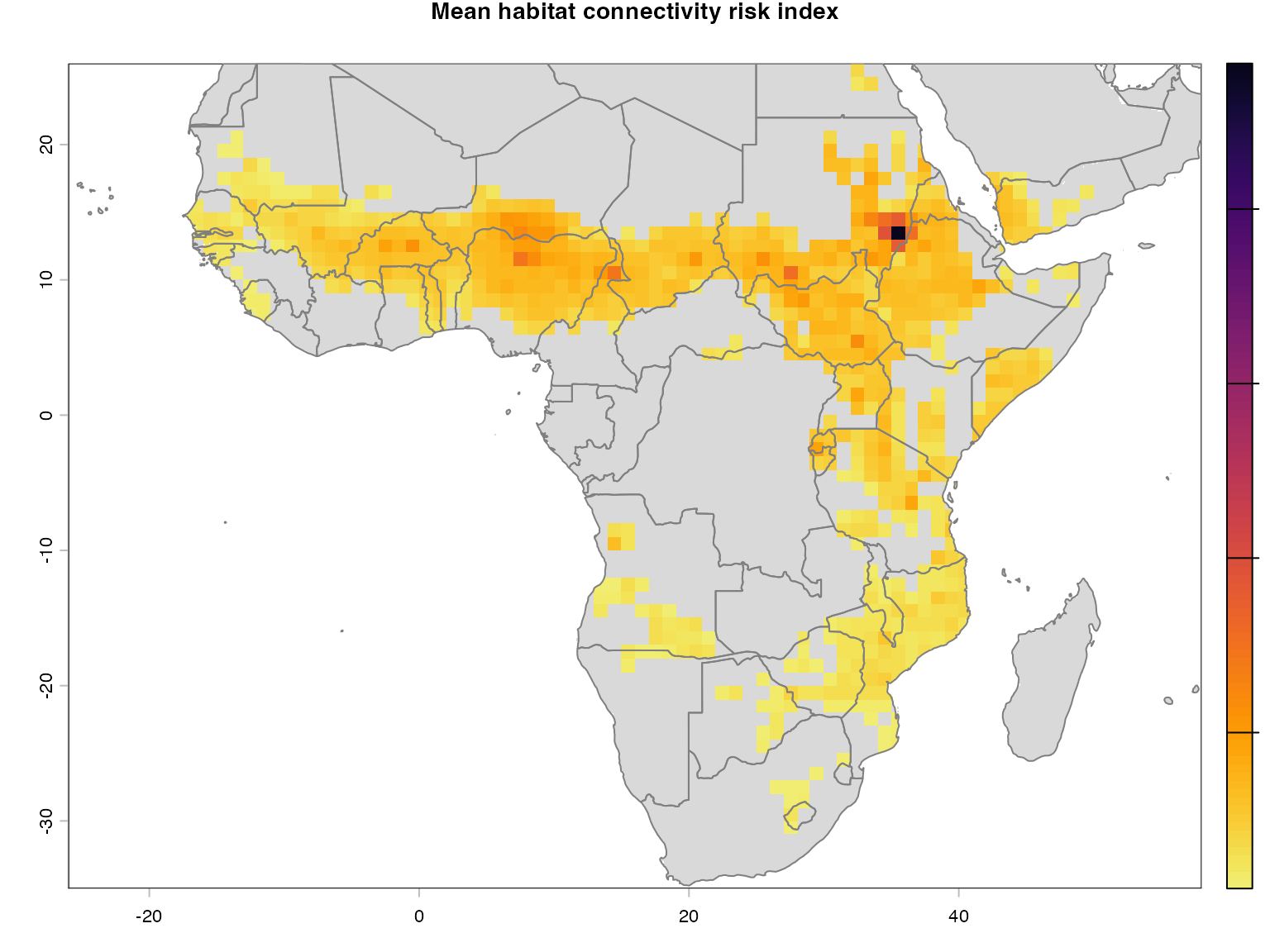

plot(sorghumland.connectivity@me_rast, col = vir.pal, 
     main = "Mean sorghumland connectivitys") #to extract the SpatRaster for mean cropland connectivivty
plot(countriesLow, add=TRUE, border = "grey25")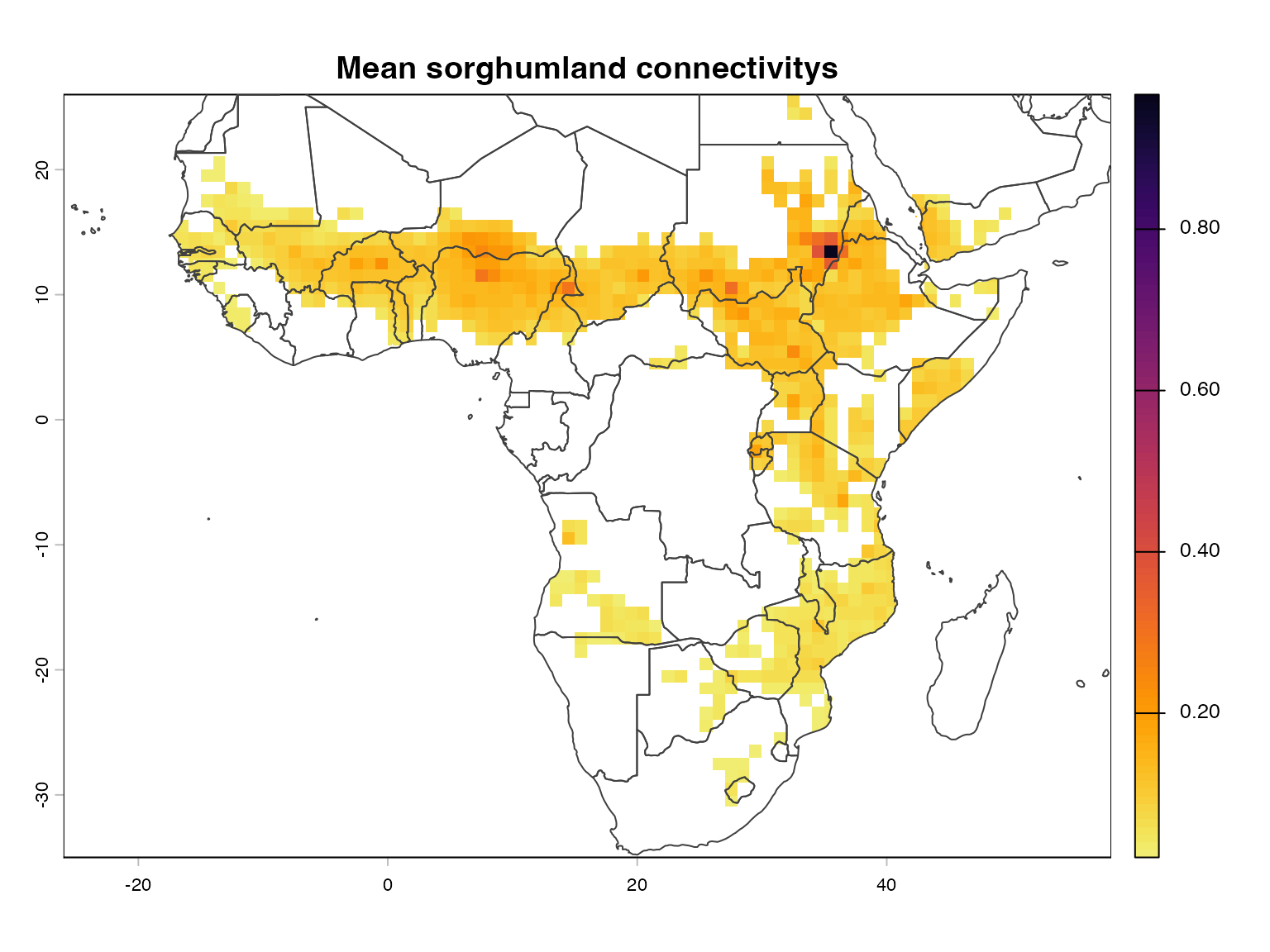

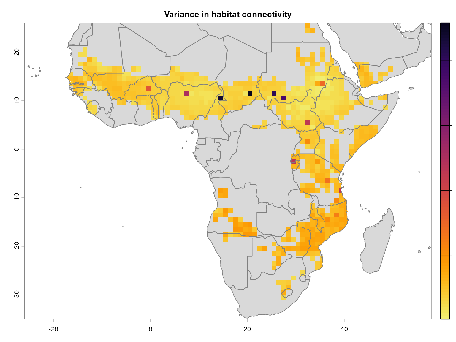
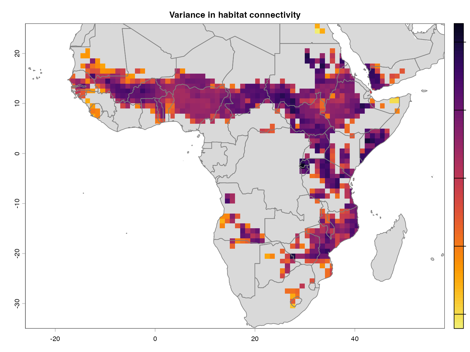
plot(sorghumland.connectivity@var_rast, col = vir.pal, 
     main = "Variance in sorghumland connectivity") #to extract the SpatRaster for variance in cropland connectivity 
plot(countriesLow, add=TRUE, border = "grey25")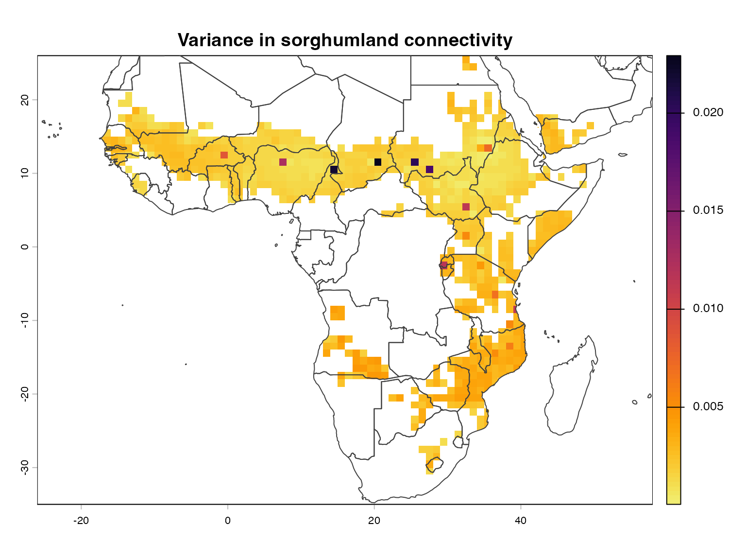

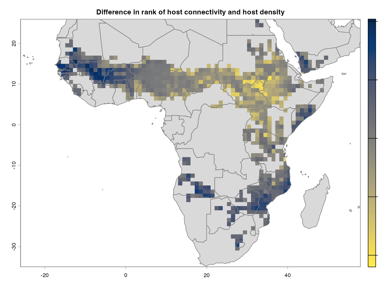
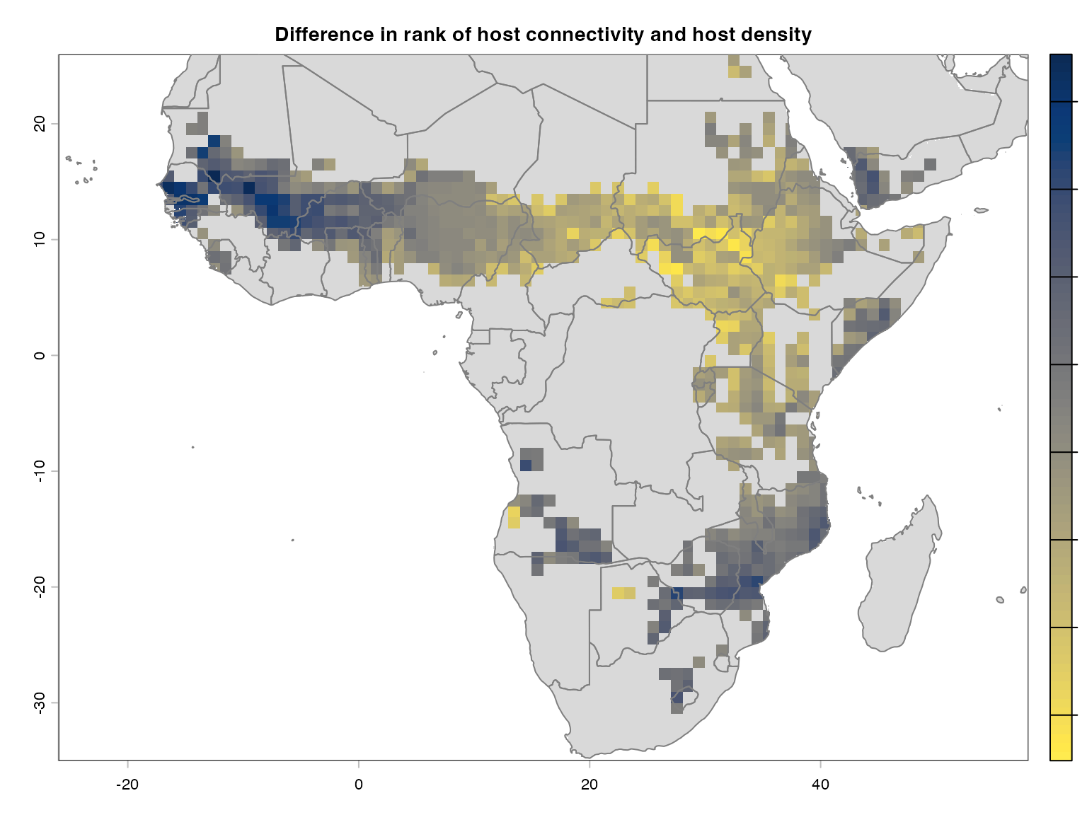
plot(sorghumland.connectivity@diff_rast, col = paldif, 
     main = "Difference between sorghumland connectivity and density") #to extract the SpatRaster for difference between mean cropland connectivity and host density
plot(countriesLow, add=TRUE, border = "grey25")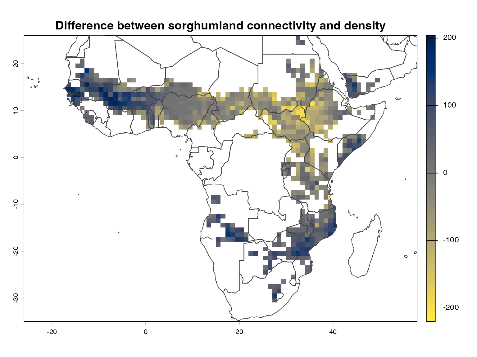

# Second analysis: customizing the parameter values
sorghumland.connectivity.clos<-msean(sorghumland.density,
                                     agg_methods = c("mean"), 
                                     dist_method = "geodesic",
                                     link_threshold =  0.00001, 
                                     hd_threshold = 0.0025,
                                     res = 12, global = FALSE, 
                                     geoscale = c(-26, 58, -35, 26),
                             inv_pl = inv_powerlaw(NULL, betas = c(0.5, 1, 1.5), mets = c("closeness",    "NODE_STRENGTH", "Sum_of_nearest_neighbors", "eigenVector_centrAlitY"), we = c(50, 15, 15, 20), linkcutoff = -1),
                             neg_exp = neg_expo(NULL, gammas = c(0.05, 1, 0.2, 0.3), mets = c("closeness",    "NODE_STRENGTH", "Sum_of_nearest_neighbors", "eigenVector_centrAlitY"), we = c(50, 15, 15, 20), linkcutoff = -1))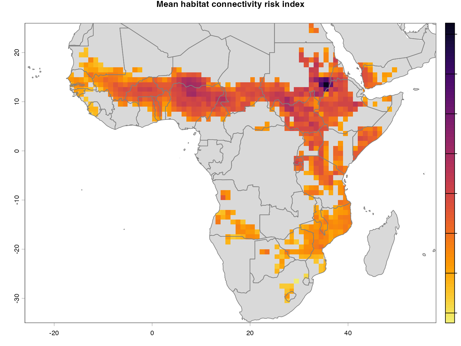

plot(sorghumland.connectivity.clos@me_rast, col = vir.pal, main = "Mean sorghumland connectivity with closeness") 
plot(countriesLow, add=TRUE, border = "grey25")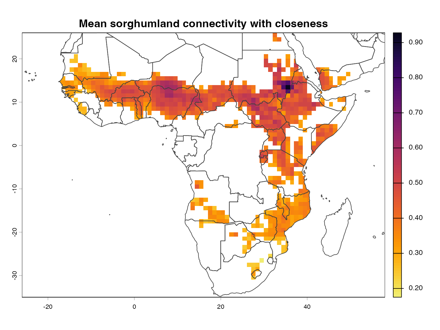

plot(sorghumland.connectivity.clos@var_rast, col = vir.pal, main = "Variance in sorghumland connectivity with closeness")
plot(countriesLow, add=TRUE, border = "grey25")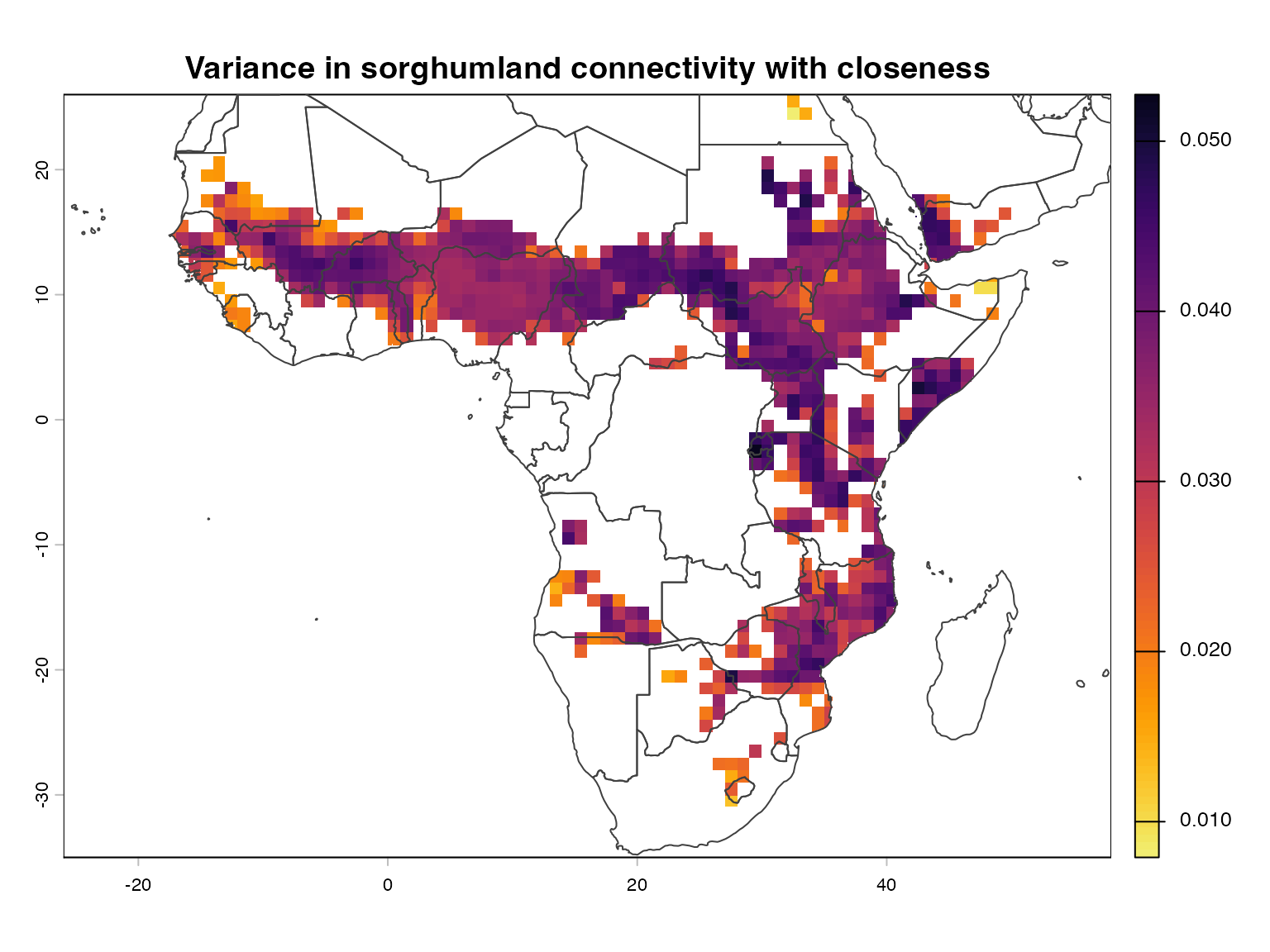

plot(sorghumland.connectivity.clos@diff_rast, col = paldif, main = "Difference between sorghumland connectivity (with closeness) and density") 
plot(countriesLow, add=TRUE, border = "grey25")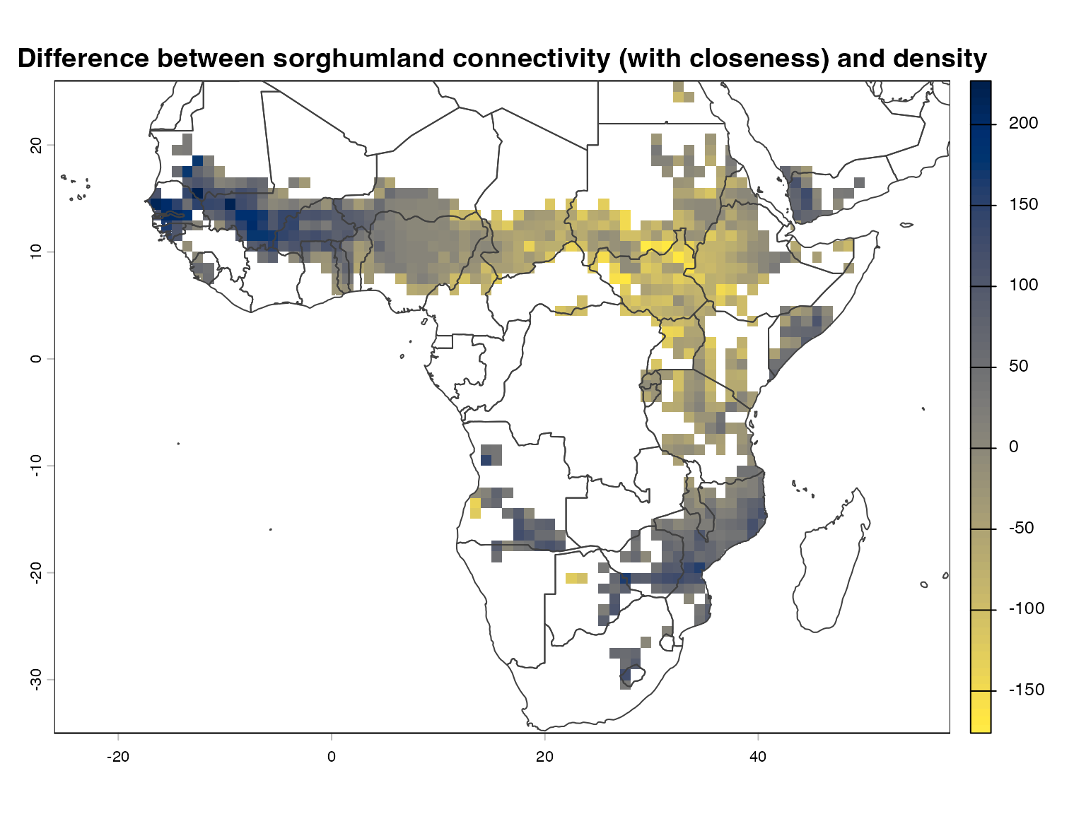

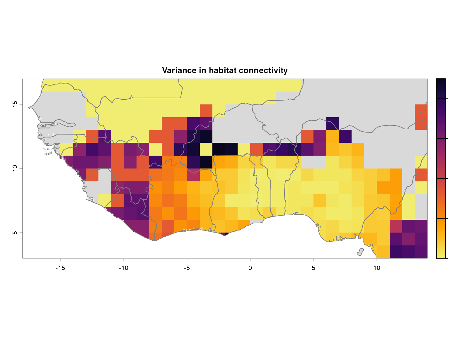
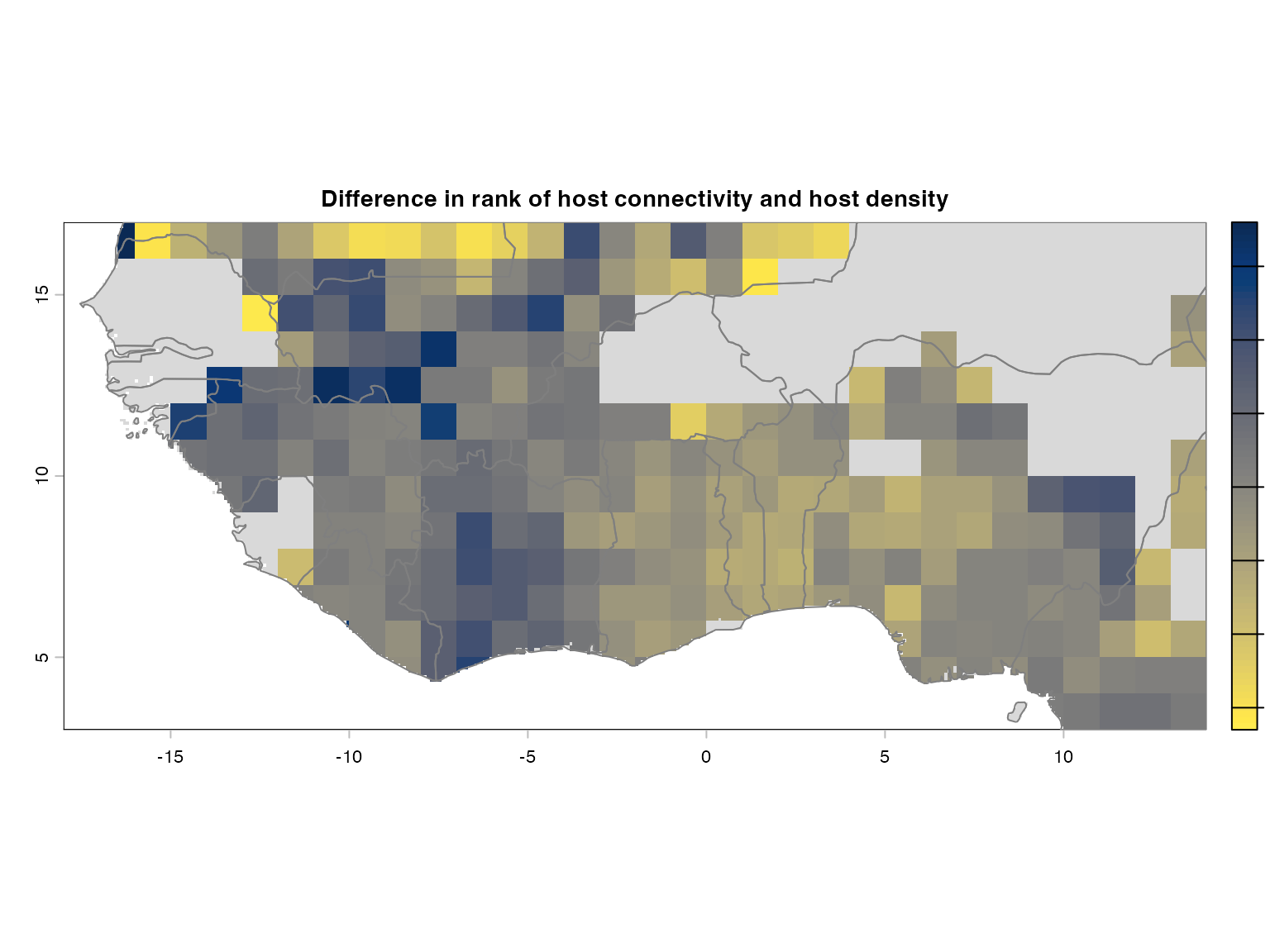
Yams landscape connectivity in the west African region

Here in the first analysis, we changed the distance calculation method, the hd_threshold value, and the rating of the four default network metrics. In the second analysis, we changed the betweeness centrality with closeness centrality

#First analysis: customizing the parameter values
  
yamsland.connectivity.betw<-msean(yamsland.density,
                                         agg_methods = c("mean"), dist_method = "vincentyellipsoid",
                                         link_threshold =  0.00001, hd_threshold = 0.00001,
                                         res = 12, global = FALSE, geoscale = c(-18, 14, 3, 17),
                             inv_pl = inv_powerlaw(NULL, betas = c(0.5, 1, 1.5), mets = c("betweeness",    "NODE_STRENGTH", "Sum_of_nearest_neighbors", "eigenVector_centrAlitY"), we = c(50, 16.67, 16.67, 16.66), linkcutoff = -1),
                             neg_exp = neg_expo(NULL, gammas = c(0.05, 1, 0.2, 0.3), mets = c("betweeness",    "NODE_STRENGTH", "Sum_of_nearest_neighbors", "eigenVector_centrAlitY"), we = c(50, 16.67, 16.67, 16.66), linkcutoff = -1))

plot(yamsland.connectivity.betw@me_rast, col = vir.pal, main = "Mean yamsland connectivity with betweensess")
plot(countriesLow, add=TRUE, border = "grey25")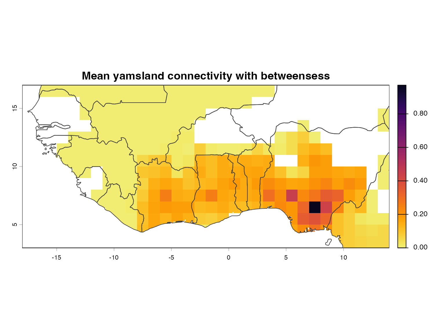

plot(yamsland.connectivity.betw@var_rast, col = vir.pal, main = "Variance in yamsland connectivity with betweensess") 
plot(countriesLow, add=TRUE, border = "grey25")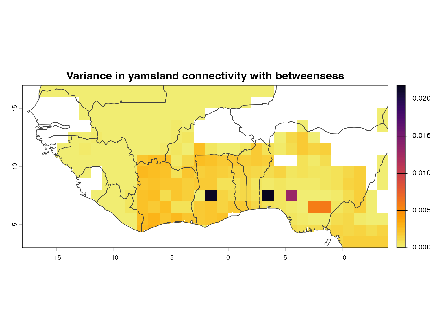

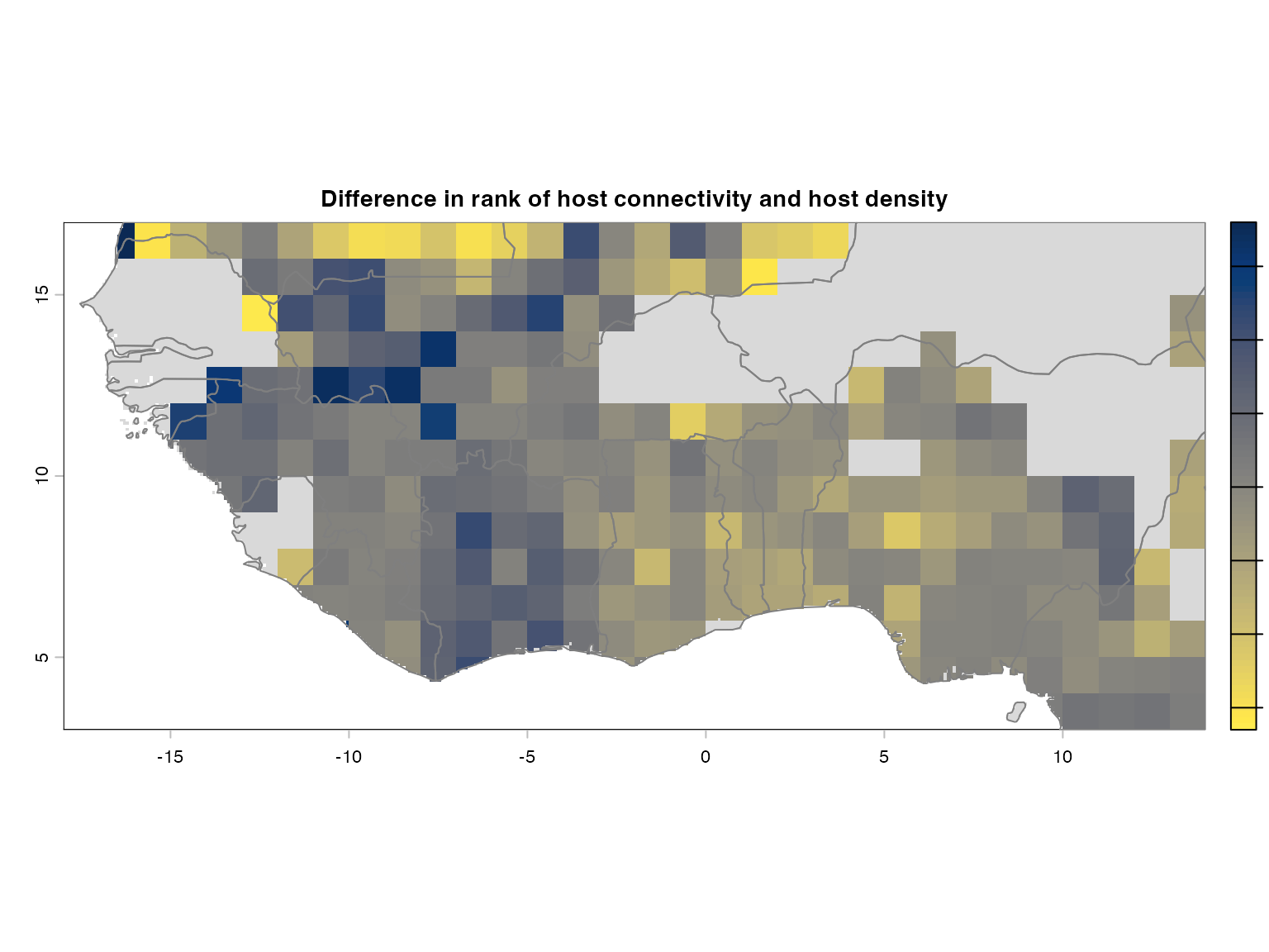
plot(yamsland.connectivity.betw@diff_rast, col = paldif, main = "Difference between yamsland connectivity (with betweensess) and density")
plot(countriesLow, add=TRUE, border = "grey25")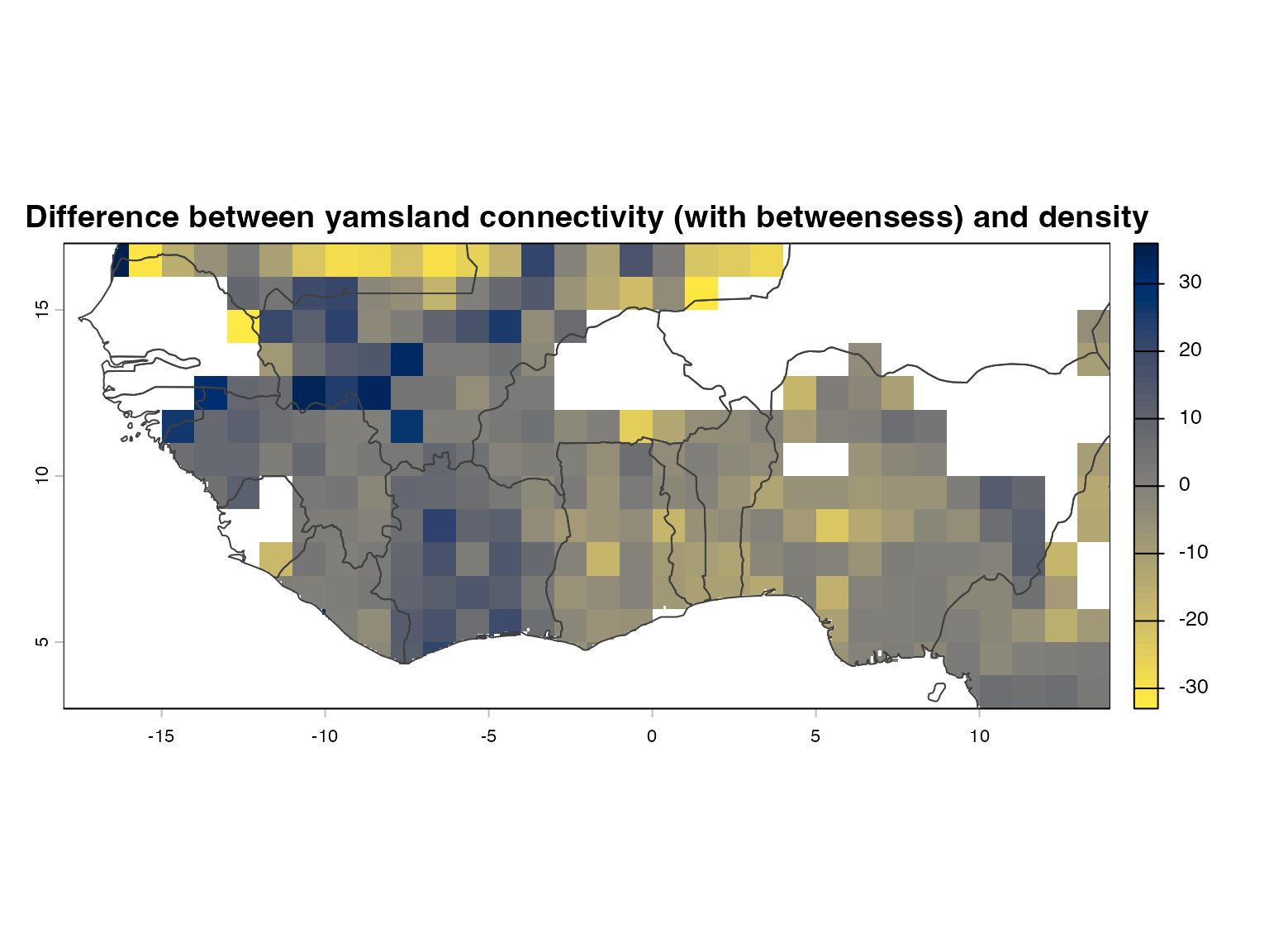

yamsland.connectivity.clos<-msean(yamsland.density,
                                         agg_methods = c("mean"), dist_method = "vincentyellipsoid",
                                         link_threshold =  0.00001, hd_threshold = 0.00001,
                                         res = 12, global = FALSE, geoscale = c(-18, 14, 3, 17),
                             inv_pl = inv_powerlaw(NULL, betas = c(0.5, 1, 1.5), mets = c("closeness",    "NODE_STRENGTH", "Sum_of_nearest_neighbors", "eigenVector_centrAlitY"), we = c(50, 16.67, 16.67, 16.66), linkcutoff = -1),
                             neg_exp = neg_expo(NULL, gammas = c(0.05, 1, 0.2, 0.3), mets = c("closeness",    "NODE_STRENGTH", "Sum_of_nearest_neighbors", "eigenVector_centrAlitY"), we = c(50, 16.67, 16.67, 16.66), linkcutoff = -1))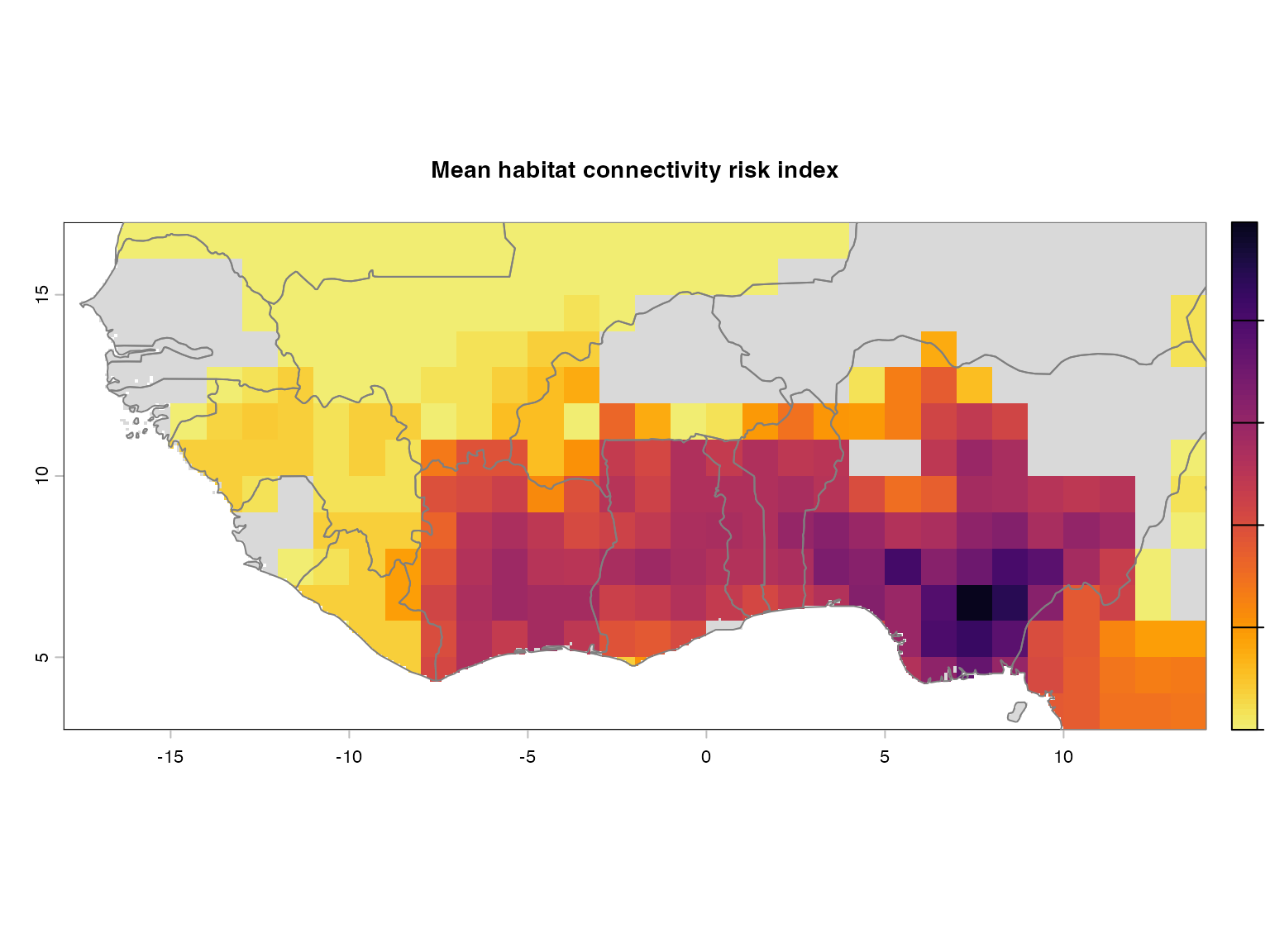

#Second analysis: customizing the parameter values

plot(yamsland.connectivity.clos@me_rast, col = vir.pal, main = "Mean yamsland connectivity with closeness") 
plot(countriesLow, add=TRUE, border = "grey25")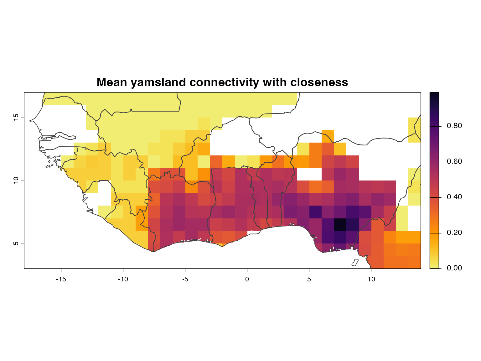

plot(yamsland.connectivity.clos@var_rast, col = vir.pal, main = "Variance in yamsland connectivity with closeness")
plot(countriesLow, add=TRUE, border = "grey25")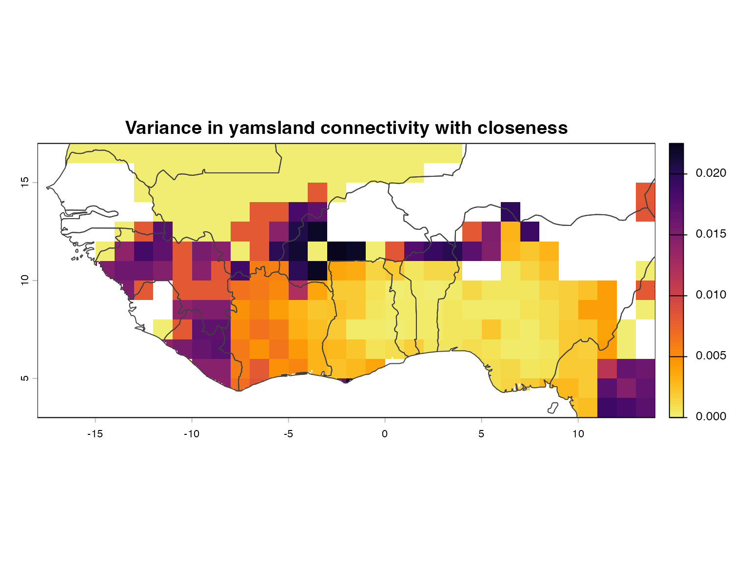

plot(yamsland.connectivity.clos@diff_rast, col = paldif, main = "Difference between yamsland connectivity (with closeness) and density") 
plot(countriesLow, add=TRUE, border = "grey25")