Case study 1

The objective of this vignette is to illustrate the underlying assumptions to calculate habitat connectivity in the geohabnet package using a simple example. If you are interested in a particular step in in the habitat connectivity analysis, you can skip some sections. However, we recommend beginners to look at the material in sequence of sections in the vignette.

Creating a hypothetical habitat landscape

The first step is to create a matrix that represent the spatial distribution of the habitat in a landscape. To do this, we create a matrix where entries are zeros (no habitat available) and then fill with a hypothetical distribution of the habitat for each cell.

We then convert this habitat matrix into a raster object with actual coordinates and plot this new raster object to show the hypothetical distribution of habitat density in the world. In this example, we simply assumed that each entry in the habitat matrix is equal to a one-degree cell in the world, with the geographic extent going from -120 to -110 in longitude (or ten columns in the matrix) and from 30 to 40 in latitude (or ten rows in the matrix).

# generating a matrix with zeros
m<-matrix(0,nrow=10, ncol=10)

# assigning non-zero values to some entries in the matrix
# Note that these values represent habitat density (usually ranging from 0 to 1)
m[3,3]<-0.1
m[3,4]<-0.1
m[3,5]<-0.2
m[3,8]<-0.1
m[3,10]<-0.1
m[6,8]<-0.1
m[10,8]<-0.1

# converting the matrix into a rast object for habitat distribution representing a map of habitat density
library(terra)

## Warning: package 'terra' was built under R version 4.5.2

## terra 1.9.27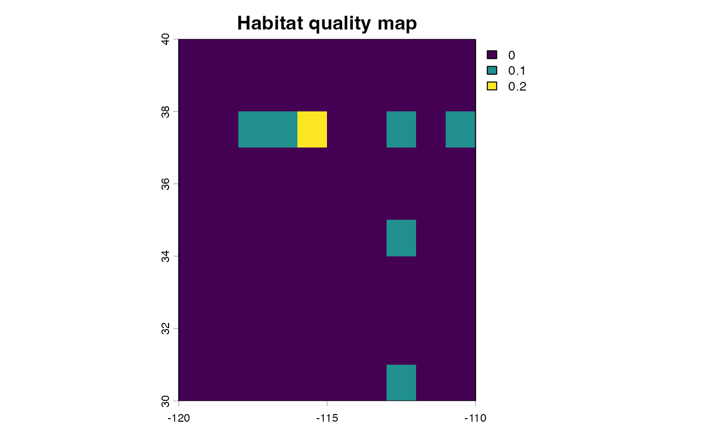

simple.rast<-rast(m, extent=c(-120,-110,30,40))
plot(simple.rast, main = "Habitat quality map")

# OPTIONAL: you can also save the generated raster in your computer for future use.
writeRaster(simple.rast, "case1.tif", overwrite=TRUE)

Note that, in practice, you may already have your map of habitat density in a raster format and you may not need to create a habitat density matrix and convert it into a raster object. For example, we have used available maps of habitat distribution from EarthStat, the Spatial Production Allocation Model and CropGrids. See other vignettes that provide information of how to use different types of data sets to generate maps of habitat density that can be used in geohabnet.

Transforming a habitat landscape into an adjacency matrix

The next step is to construct an adjacency matrix, in which rows represent source locations, columns represent destination locations, and entry values indicate the relative likelihood of pathogen spreading from one location to another. We will use the previously created map of habitat density.

# Getting the longitude and latitude of each cell in the landscape that has a habitat density greater than a habitat density threshold (in this case, values greater than zero).
# This selection of cells helps us to focus the analysis in most important habitat locations in the landscape
habitat.threshold <-0
nonZero <- which(values(simple.rast)>habitat.threshold) #this gets cells that have non-zero values
latilongimatr <- xyFromCell(simple.rast, cell = nonZero) #this calculate the geographic coordinates of specified cells, where x represents longitude and y represents latitude

# Generating a DISTANCE matrix, in which each row or column represents a cell in the habitat landscape with a habitat population greater than the specified threshold above, and each entry is the geographic distance between a pair of habitat cells
library(geosphere)

## Warning: package 'geosphere' was built under R version 4.5.2

distMat <- matrix(-999, nrow(latilongimatr), nrow(latilongimatr)) #this generates a matrix with a constant values, which is set to -999 here
dvse <- geosphere::distVincentyEllipsoid(c(0,0), cbind(1, 0)) #this calculates the distance (in meters) between two cells of one degree at the equators, which is used in our analysis for scaling distances
for (i in 1:nrow(latilongimatr)) {
      distMat[i, ] <- distVincentyEllipsoid(latilongimatr[i,], latilongimatr)/dvse
} #this calculates the distance between every pair of selected habitat cells

# Generating a DISPERSAL matrix, in which each row or column represents a cell in the habitat landscape with a habitat population, and each entry is the probability of pest moving between a pair of habitat cells. In this hypothetical example, the pest movement probability is based on a commonly used dispersal kernel: the inverse power law model.
beta<-0.7 #the beta parameter in the inverse power law model, which can be determined empirically
distPL<-distMat^(-beta) #the inverse power law model

# Generating a habitat matrix, in which each row or column represent a cell in the habitat landscape, and each entry is the product of habitat densities between each pair of habitat cells
habitat.density <- values(simple.rast)[nonZero]
habitatmatr1 <- matrix(habitat.density, , 1 )
habitatmatr2 <- matrix(habitat.density, 1, )
habitatmatrix <- habitatmatr1 %*% habitatmatr2 
habitatmatrix <- as.matrix(habitatmatrix)

# Generating a matrix that represent the relative likelihood of pathogen movement between each pair of habitat locations or habitat cells in the landscape, accounting for both dispersal kernel and habitat availability
habitatdistancematr <- distPL * habitatmatrix #this is the gravity model for habitat density

# Focusing the analysis by 'removing' entries in the previous matrix that have a relative likelihood smaller than 0.004
# This link threshold is an arbitrary threshold value, but it helps to focus the analysis on major connections
link.threshold <- 0.004 
logimat <- habitatdistancematr>link.threshold
habitatdistancematr<-habitatdistancematr*logimat
class(habitatdistancematr)

## [1] "matrix" "array"

# Check this adjacency matrix of the relative likelihood of pest moving between habitat locations
habitatdistancematr

##            [,1]        [,2]        [,3]        [,4]        [,5]        [,6]
## [1,]        Inf 0.011748900 0.014464735 0.000000000 0.000000000 0.000000000
## [2,] 0.01174890         Inf 0.023497800 0.004452221 0.000000000 0.000000000
## [3,] 0.01446474 0.023497800         Inf 0.010890649 0.007616975 0.007780485
## [4,] 0.00000000 0.004452221 0.010890649         Inf 0.007232368 0.004645163
## [5,] 0.00000000 0.000000000 0.007616975 0.007232368         Inf 0.004245301
## [6,] 0.00000000 0.000000000 0.007780485 0.004645163 0.004245301         Inf
## [7,] 0.00000000 0.000000000 0.004924583 0.000000000 0.000000000 0.000000000
##             [,7]
## [1,] 0.000000000
## [2,] 0.000000000
## [3,] 0.004924583
## [4,] 0.000000000
## [5,] 0.000000000
## [6,] 0.000000000
## [7,]         Inf

So the adjacency matrix printed above is ready to be converted into a network. It is important to check some attributes of this adjacency matrix before converting this into a graph object.

All the diagonal entries are set to Inf because they represent the probability of pathogen movement to that same habitat location in the landscape, which is infinite and is not included in further analysis below.
This adjacency matrix is square because the number of rows is equal to the number of columns.
This adjacency matrix is symmetric. For example, the relative likelihood of a pathogen moving from location 1 to location 2 is the same as moving from location 2 to location 1. This means that this adjacency matrix can be used to create an undirected graph or network.

Transforming an adjacency matrix into a network

Note: A graph object is the name for a network in the igraph package in R.

library(igraph)

# Generating a graph object from an adjacency matrix
habitatnet <- graph.adjacency(habitatdistancematr,
                           mode=c("undirected"), 
                           diag=F, #excluding entries in the diagonal
                           weighted=T) #entries will be considered link weights in the network
# Checking the content of the graph object
habitatnet

## IGRAPH 94383c7 U-W- 7 11 -- 
## + attr: weight (e/n)
## + edges from 94383c7:
##  [1] 1--2 1--3 2--3 2--4 3--4 3--5 3--6 3--7 4--5 4--6 5--6

# Visualizing the graph object
plot(habitatnet, edge.width = E(habitatnet)$weight*500, main = "Habitat network")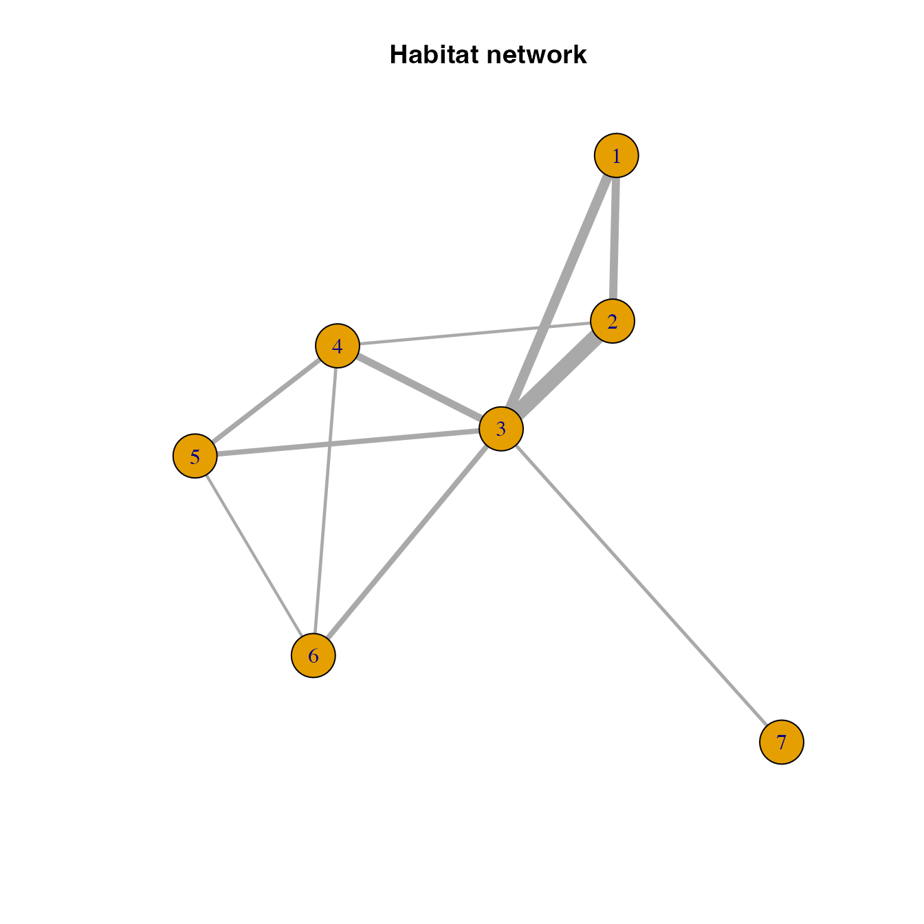

In this network, nodes represent the selecte habitat locations and links (or connections) represent the likely movement betwen any pair of locations.

We usually call this a pest invasion or epidemic network because this represents the likely movement of a pest or pathogen based on habitat availability and physical proximity. Note also that if you include other risk factors (such as climate suitability) when calculating the probability of movement between locations, you could also call this a habitat network.

Calculating the connectivity of nodes in a habitat network

There are multiple ways to calculate the connectivity of nodes in a network. These ways are often referred to as network metrics or node centralities. We can use a network metric to measure the importance of a habitat location (or node) in an invasion, epidemic or habitat network. Each network metric provides a different perspective of the potential role of a node during an epidemic, invasion or the spread of a species. Below, we illustrate three commonly used network metrics for the hypothetical example.

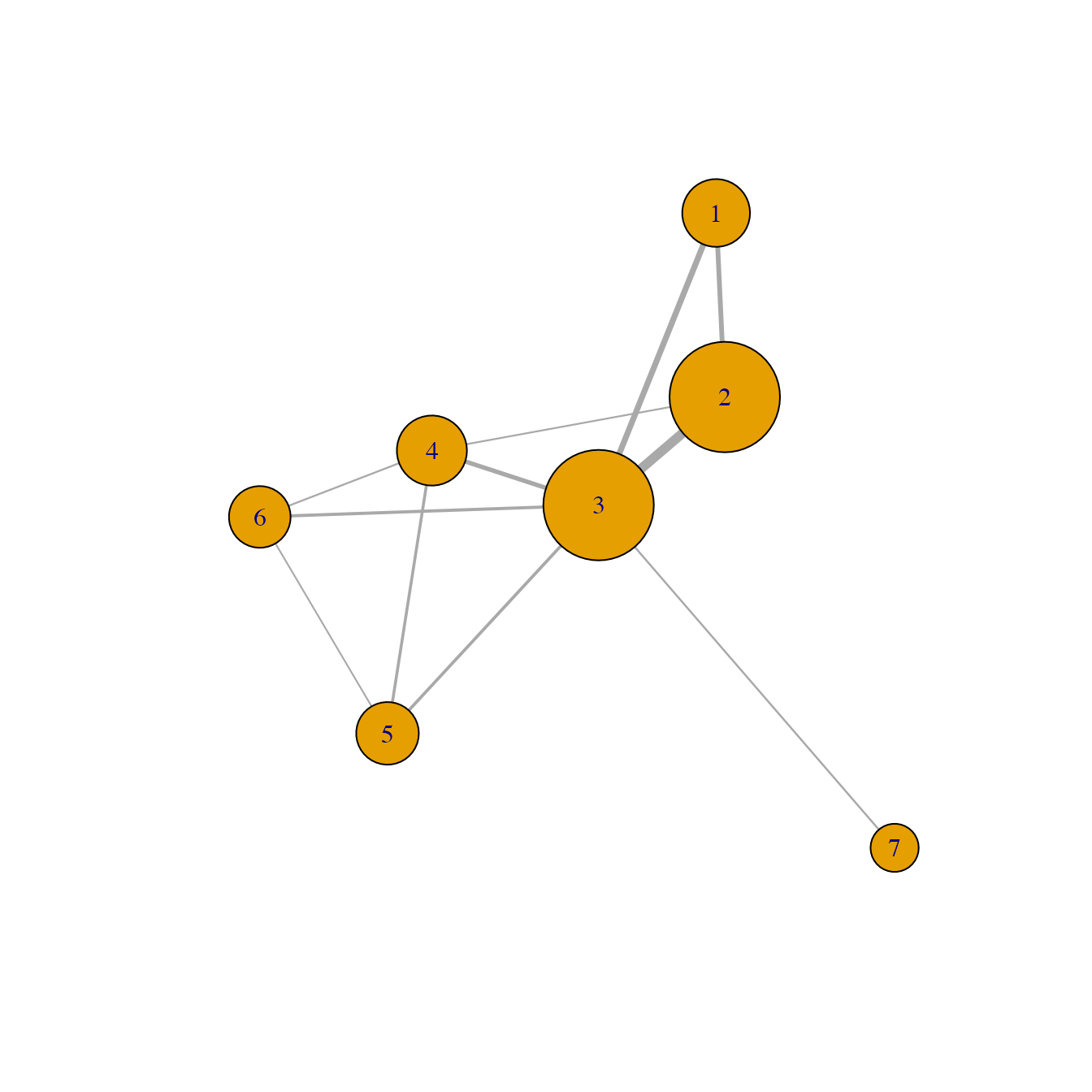
habitat location importance based on node strength

# Calculating the node strength of habitat locations in the network
V(habitatnet)$strength <- strength(habitatnet, weights = E(habitatnet)$weight)
# Visualizing the importance of habitat nodes in the habitat network using node size
# The larger the node, the more important the node in the habitat network
plot(habitatnet, #this is the graph object to plot
     vertex.size = V(habitatnet)$strength*500, #making vertex size in the plot proportional to node strength in the graph object
     edge.width = E(habitatnet)$weight*500, #making link width in the plot proportional to edge weights in the graph object
     main = "Node strength")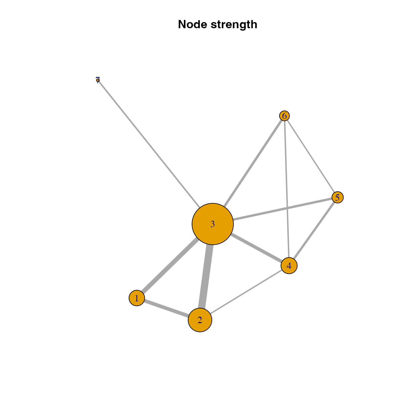

habitat location importance based on eigenvector centrality

# Calculating and visualizing the eigenvector centrality of habitat locations in the network
V(habitatnet)$evcent <- eigen_centrality(habitatnet)$vector
plot(habitatnet, vertex.size = V(habitatnet)$evcent*40, 
     edge.width = E(habitatnet)$weight*500, main = "Eigenvector centrality")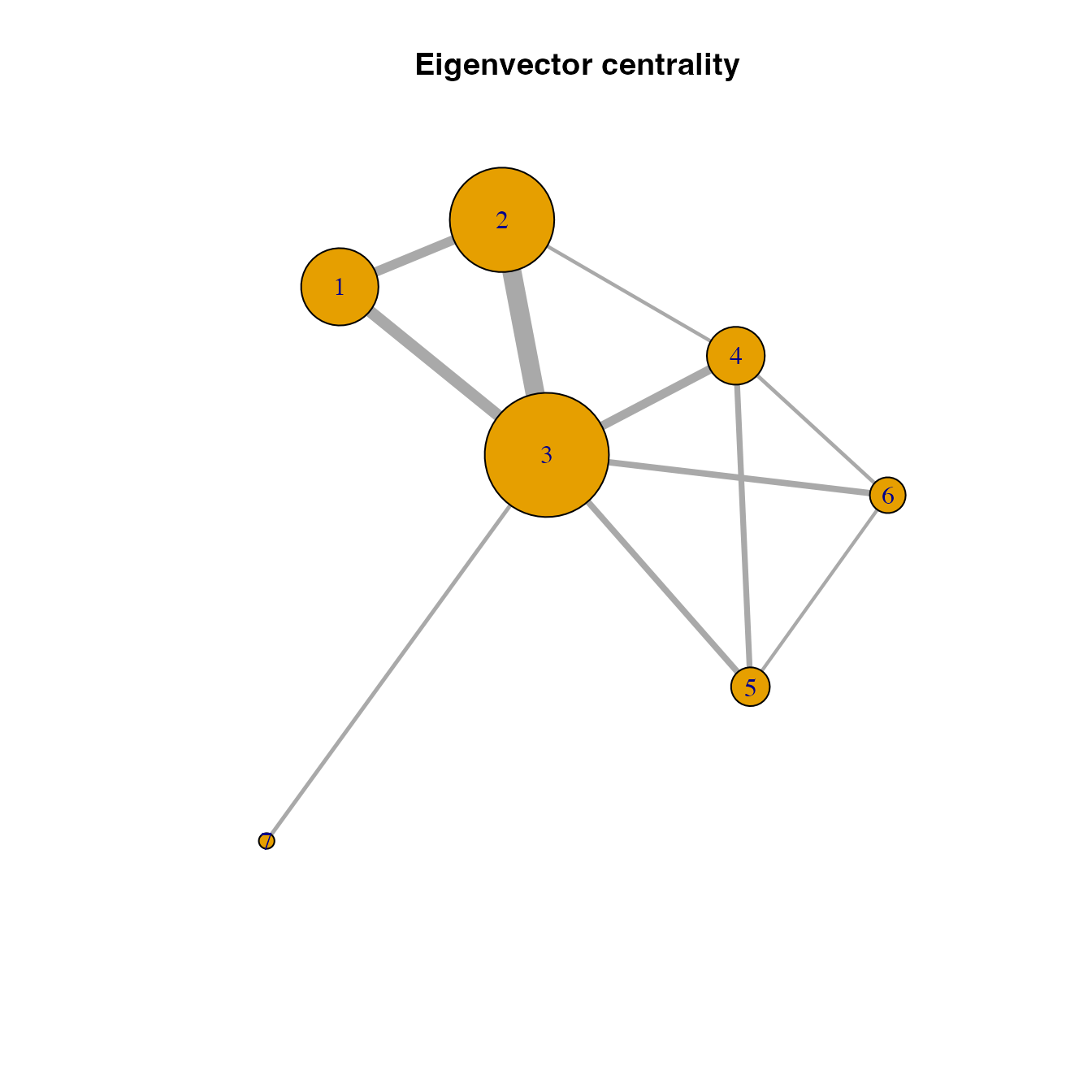

Betweenness centrality

Did you realize that we provided the link weights in the function when calculating node strength but not so when calculating eigenvector centrality? Well, in this case, either way is okay because the graph object has only ony type of links and the interpretation of link weights in both node centrality measures is in line with our expectation of pest movement: higher link weights is directly proportional to higher likelihood of pest movement.

This interpretation is not valid for the betweenness function in igraph, where link weights are interpreted as distances to calculate the shortest paths. This interpretation is the opposite and wrong to what we would expect to occur in a invasion network: higher link weights means longer distances and lower likelihood of pest movement. Instead, our analysis should correctly match the shortest paths with those paths where pest movement is most likely (i.e., higher link weights). So, we need to transform so that new link weights are inversely proportional to the likelihood of pest movement when calculating betweenness centrality.

Note that this link weight transformation is needed when calculating betweenness and closeness centrality because they both depend on shortest distance for the importance of locations.

# Transforming link weights for shortest paths
trans.links<-1.0001*max(E(habitatnet)$weight)-E(habitatnet)$weight

# Calculating betweenness centrality of habitat locations in the network
V(habitatnet)$betweenness <- igraph::betweenness(habitatnet, weights = trans.links, directed = FALSE)

plot(habitatnet, vertex.size = V(habitatnet)$betweenness*2, 
     edge.width = E(habitatnet)$weight*500, main = "Node betweenness centrality")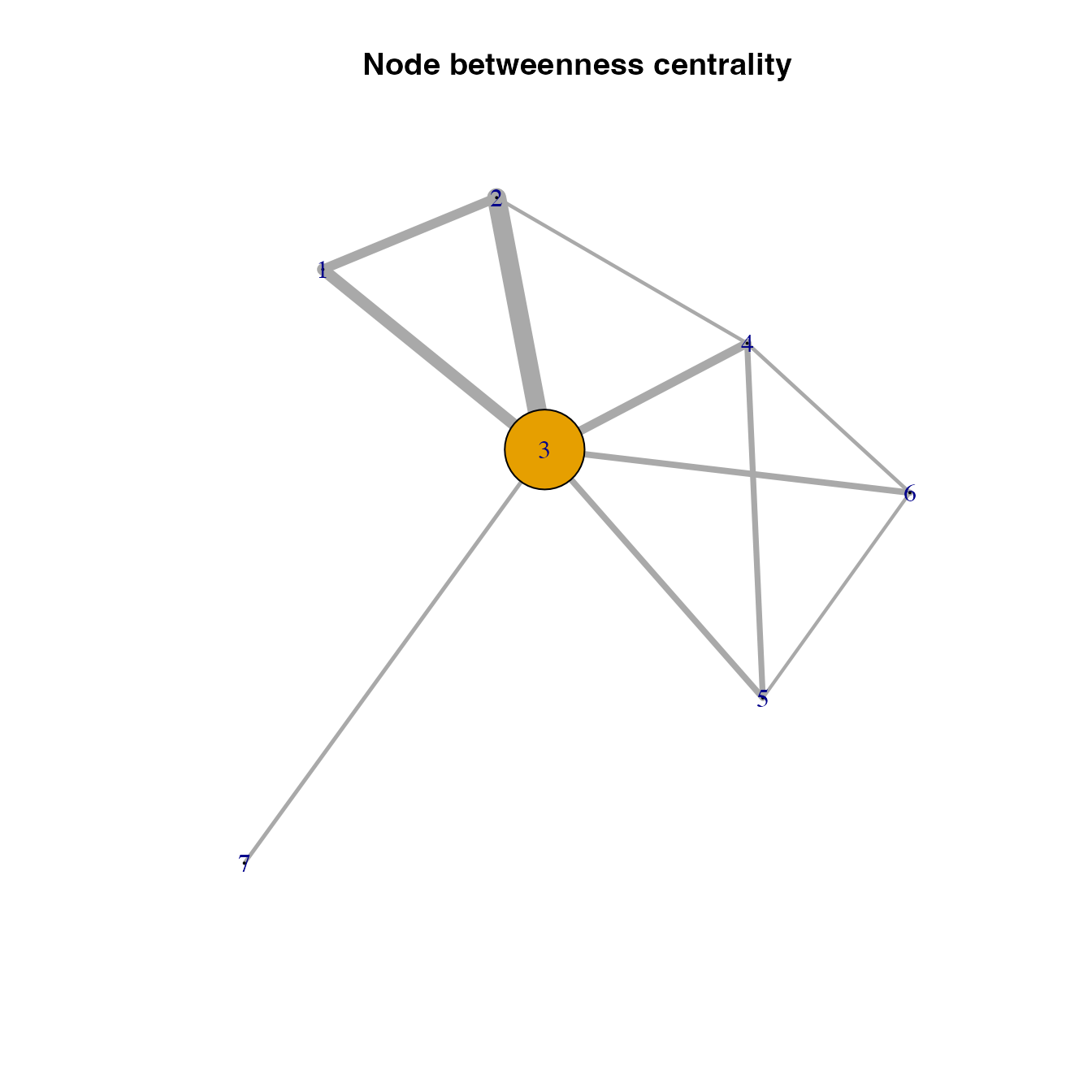

Closeness centrality

V(habitatnet)$closeness <- igraph::closeness(habitatnet, weights = trans.links)
plot(habitatnet, vertex.size = V(habitatnet)$closeness*2.5, edge.width = E(habitatnet)$weight*250)

Generating maps of surveillance prioritization based on the importance of habitat locations

Now that we have applied a network analysis to our habitat distribution data, we can generate maps of surveillance priorities for each network metric or a combination of them. This process consists of simply assigning or matching the importance of habitat locations based on a network metric to the specified locations in the habitat density map (or any raster object with the same geographic attributes, that is, number of cells, geographic extent, and spatial resolution).

# Generating a raster object
closeness.rast<-simple.rast
# Assigning the betweenness centrality to each location in the map
values(closeness.rast)[nonZero]<-V(habitatnet)$closeness

# Doing the same for the other node centralities
betweenness.rast<-simple.rast
values(betweenness.rast)[nonZero]<-V(habitatnet)$betweenness

strength.rast<-simple.rast
values(strength.rast)[nonZero]<-V(habitatnet)$strength

eigen.rast<-simple.rast
values(eigen.rast)[nonZero]<-V(habitatnet)$evcent

# Plotting the location importance based on different network metrics
par(mfrow = c(2,2))
plot(strength.rast, main = "Node stregth")
plot(eigen.rast, main = "Eigenvector centrality")
plot(betweenness.rast, main = "Betweenness centrality")
plot(closeness.rast, main = "Closeness centrality")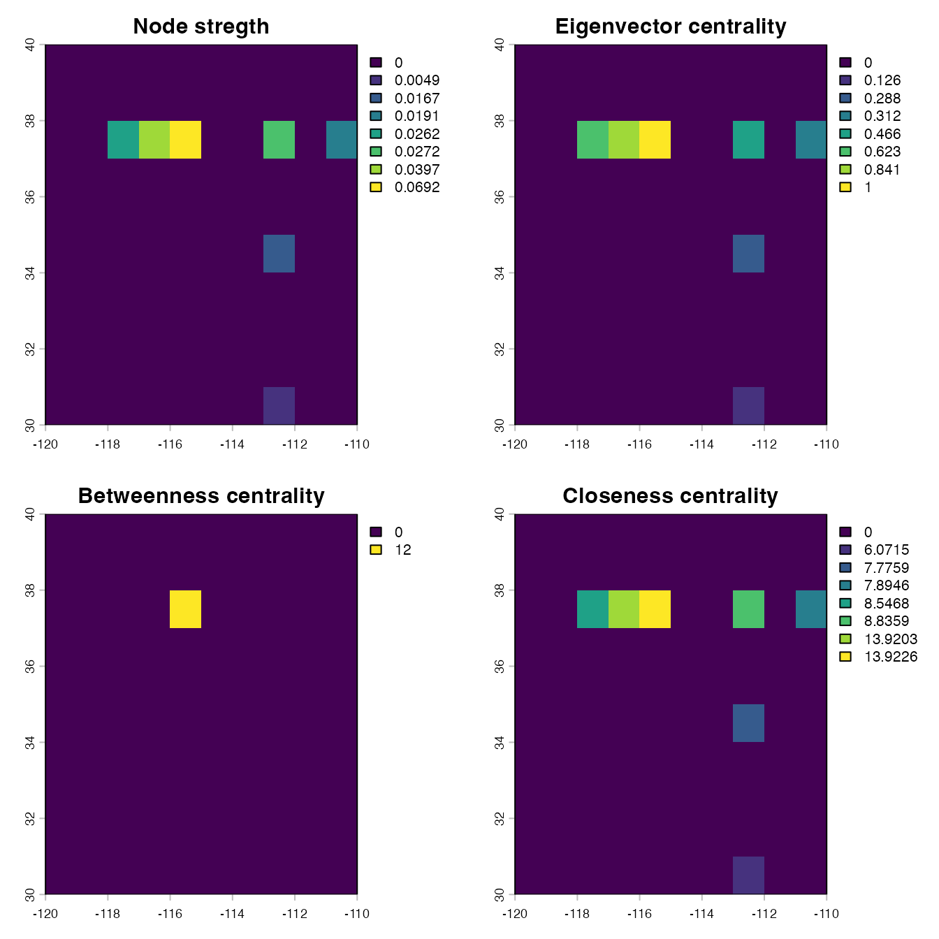

Another example for betweennes centrality

Here, we provide simpler example illustrating how betweenness centrality works. Since betweenness centrality is based on shortest paths between locations, it is difficult to get an intuition of whether those links highly weighted correctly correspond with the shortest paths. This idea is confirmed in the following example in which a network consists of four nodes, showing that node 3 is the location with the highest betweenness centrality (as expected).

new.matrix<-matrix(0,nrow=4, ncol=4)
new.matrix[2,1]<-0.1
new.matrix[3,1]<-0.5
new.matrix[1,2]<-0.1
new.matrix[4,2]<-0.1
new.matrix[2,4]<-0.1
new.matrix[3,4]<-0.5
new.matrix[1,3]<-0.5
new.matrix[4,3]<-0.5

new.graph<-graph.adjacency(new.matrix,mode=c("undirected"),diag=F,weighted=T)

V(new.graph)$betweenness <- igraph::betweenness(new.graph, weights = log(1/E(new.graph)$weight), directed = FALSE)
V(new.graph)$betweenness

## [1] 0.5 0.0 1.0 0.5

plot(new.graph, vertex.size = V(new.graph)$betweenness*50, 
     edge.width = E(new.graph)$weight*20, main = "A quick intuition for betweenness centrality")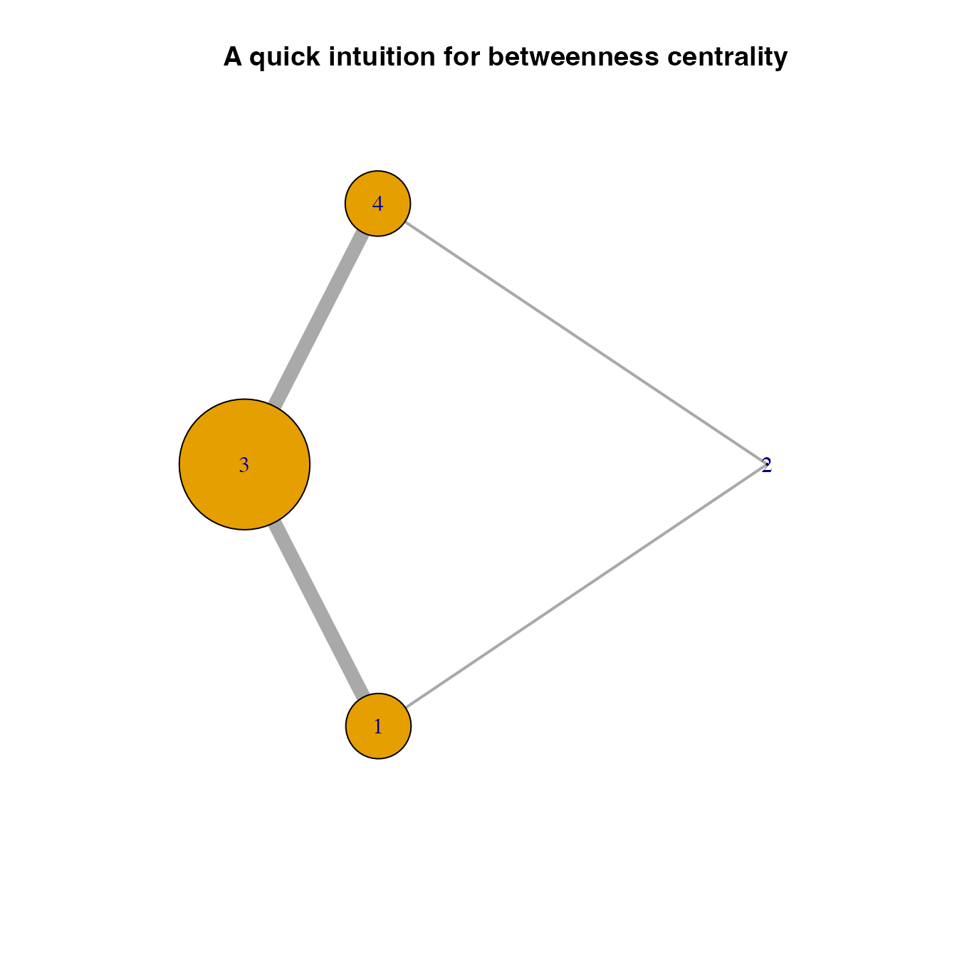

Reproducing the cartoon example from Xing et al. (2020)

Xing et al (2020) provided the foundation for the mathematical framework we used in geohabnet to conduct a habitat connectivity analysis. Figure 3 in that paper illustrates cropland connectivity for a simple hypothetical example. Let’s try to replicate this network using the knowledge you get above.

set.seed(3)
library(viridis)

## Loading required package: viridisLite

## Warning: package 'viridisLite' was built under R version 4.5.2

vir.pal<-viridis(n=100, option = "inferno", direction = -1, begin = 0.2, end = 0.9)

# getting the habitat density map
xing.mat<-system.file("extdata", "xing_cartoon.csv", package = "geohabnet")
xing.mat <- read.csv(xing.mat)
#xing.mat<-read.csv("Xing et al cartoons.csv") #
xing.mat<-as.matrix(xing.mat)
xing.rast<-rast(xing.mat, extent=c(-117,-110,33,38))
crs(xing.rast)<-"OGC:CRS84" #this assign a coordinate reference system to the raster
coords <- terra::xyFromCell(xing.rast, 1:terra::ncell(xing.rast))
node.id <- c(NA,    NA, NA, NA, 1,  2,  3,
             NA,    NA, NA, NA, 4,  5,  6,
             7, 8,  9,  10, 11, 12, 13,
             14,    15, 16, NA, NA, NA, NA,
             17,    18, 19, NA, NA, NA, NA)

plot(xing.rast, col = vir.pal, colNA = "grey85",
     main = "A) Hypothetical map of habitat suitability")
text(coords, labels = node.id, cex = 1.5, 
     col = c(rep("black",28), "white", rep("black", 6)))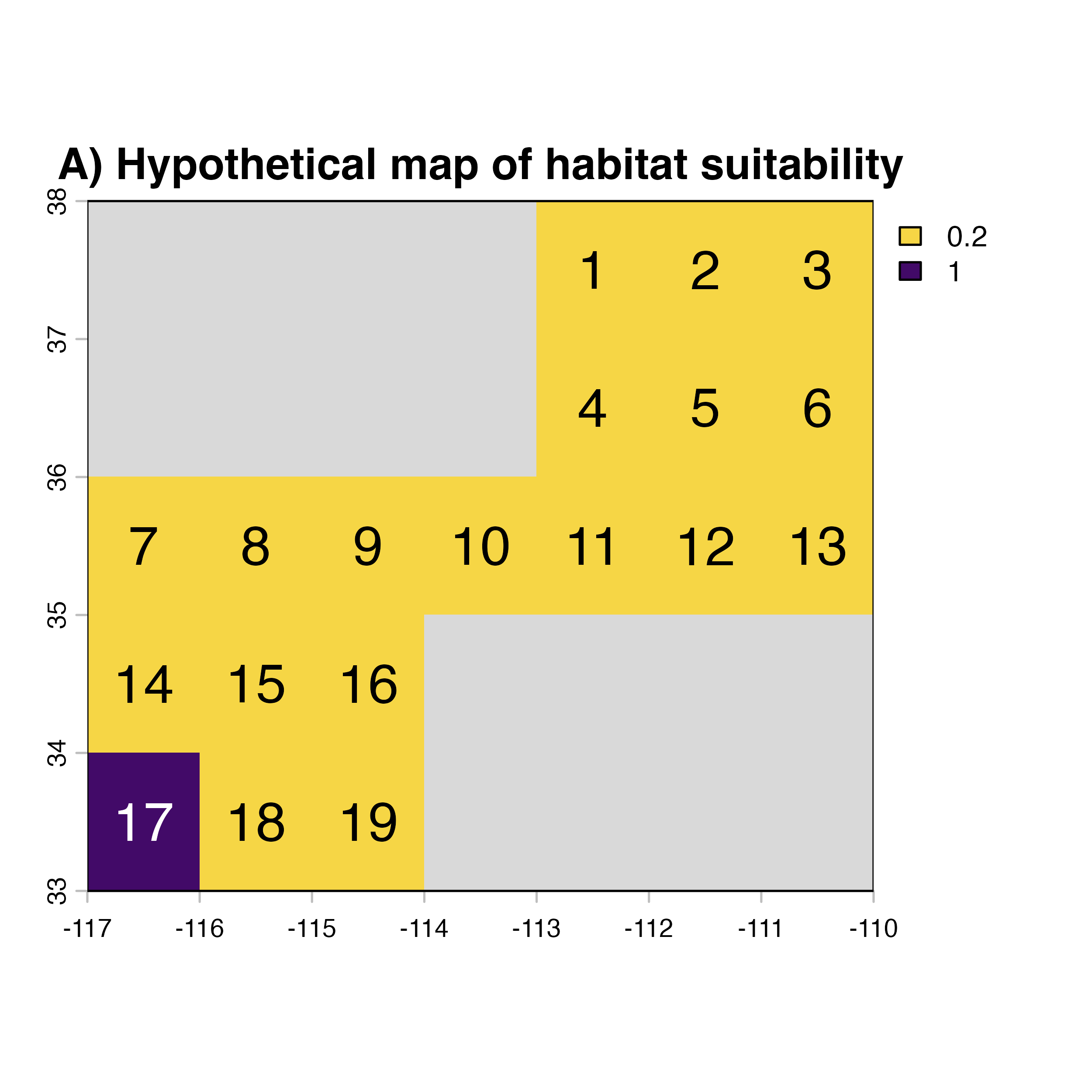

# conducting the connectivity analysis
nonZero <- which(values(xing.rast)>0)
latilongimatr <- xyFromCell(xing.rast, cell = nonZero)
distMat <- matrix(-999, nrow(latilongimatr), nrow(latilongimatr))
dvse <- geosphere::distVincentyEllipsoid(c(0,0), cbind(1, 0))
for (i in 1:nrow(latilongimatr)) {
      distMat[i, ] <- distVincentyEllipsoid(latilongimatr[i,], latilongimatr)/dvse
}
gamma <- 0.5
distPL<- exp(-1 * gamma * distMat)

habitat.density <- values(xing.rast)[nonZero]
habitatmatr1 <- matrix(habitat.density, , 1 )
habitatmatr2 <- matrix(habitat.density, 1, )
habitatmatrix <- habitatmatr1 %*% habitatmatr2
habitatmatrix <- as.matrix(habitatmatrix)

habitatdistancematr <- distPL * habitatmatrix
logimat<-habitatdistancematr>0.02
habitatdistancematr<-habitatdistancematr*logimat
habitatnet <- graph_from_adjacency_matrix(habitatdistancematr,
                                       mode=c("undirected"),diag=F,weighted=T)

## Warning: The `adjmatrix` argument of `graph_from_adjacency_matrix()` must be symmetric
## with mode = "undirected" as of igraph 1.6.0.
## ℹ Use mode = "max" to achieve the original behavior.
## This warning is displayed once per session.
## Call `lifecycle::last_lifecycle_warnings()` to see where this warning was
## generated.

V(habitatnet)$col<-c(rep("#F6D645FF",16),"#420A68FF",rep("#F6D645FF",2))
V(habitatnet)$colab<-c(rep("black",16),"white",rep("black",2))
laynet<-layout.fruchterman.reingold(habitatnet)

## Warning: `layout.fruchterman.reingold()` was deprecated in igraph 2.1.0.
## ℹ Please use `layout_with_fr()` instead.
## This warning is displayed once per session.
## Call `lifecycle::last_lifecycle_warnings()` to see where this warning was
## generated.

# plotting the pest invasion network
plot(habitatnet, edge.width = E(habitatnet)$weight*40,
     vertex.color = V(habitatnet)$col,
     vertex.label.color = V(habitatnet)$colab,
     vertex.frame.color = V(habitatnet)$col,
     layout = laynet* (-1),
     main = "B) Estimated movement network")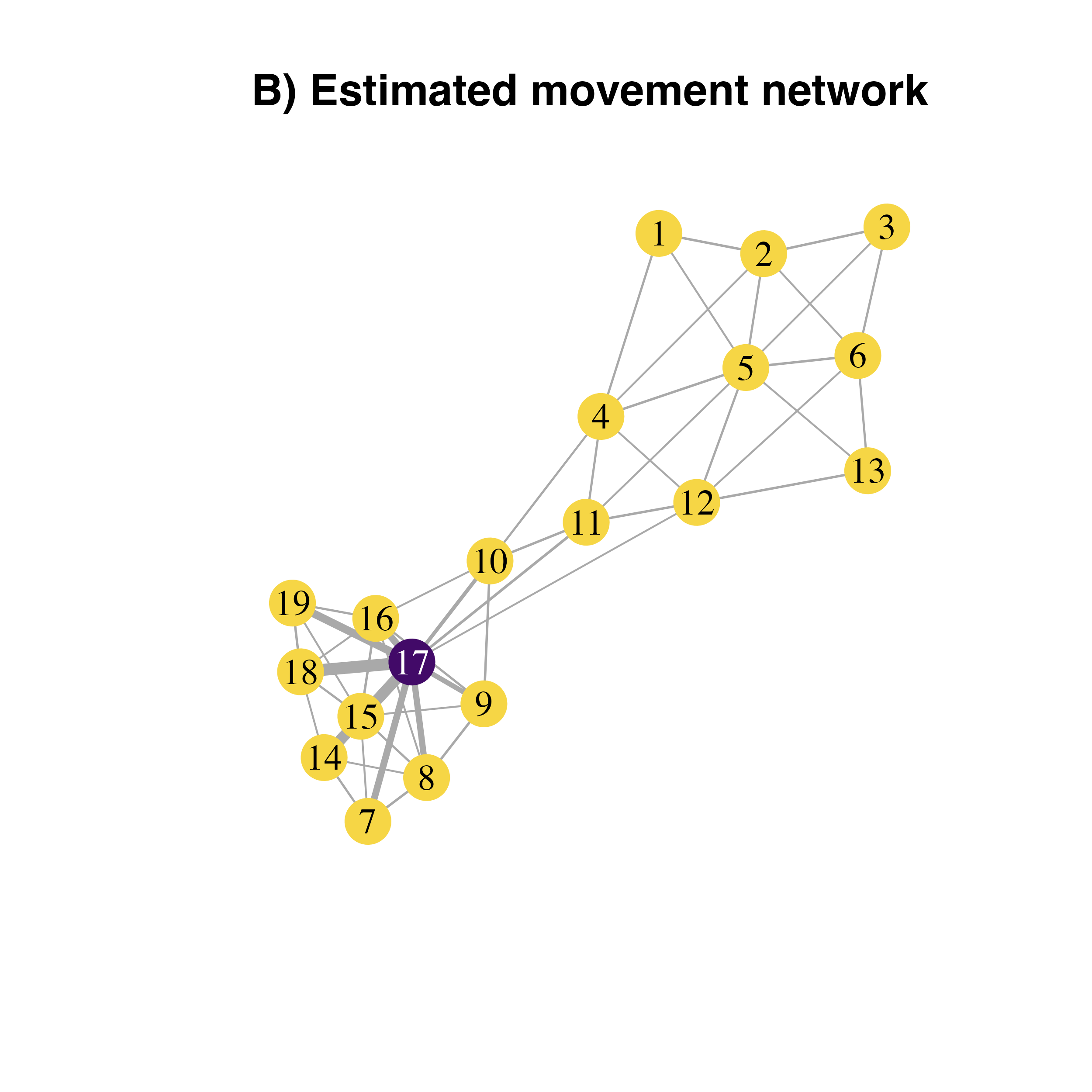

transformed.weights<-1.0001*(max(E(habitatnet)$weight))-E(habitatnet)$weight
V(habitatnet)$closeness<-closeness(habitatnet, weights = transformed.weights)

# plotting the pest invasion network with node importance
plot(habitatnet, edge.width = E(habitatnet)$weight*30, 
     vertex.size = V(habitatnet)$closeness*45,
     vertex.color = V(habitatnet)$col,
     vertex.label.color = V(habitatnet)$col,
     vertex.frame.color = V(habitatnet)$col,
     layout = laynet,
     main = "B) Estimated movement network")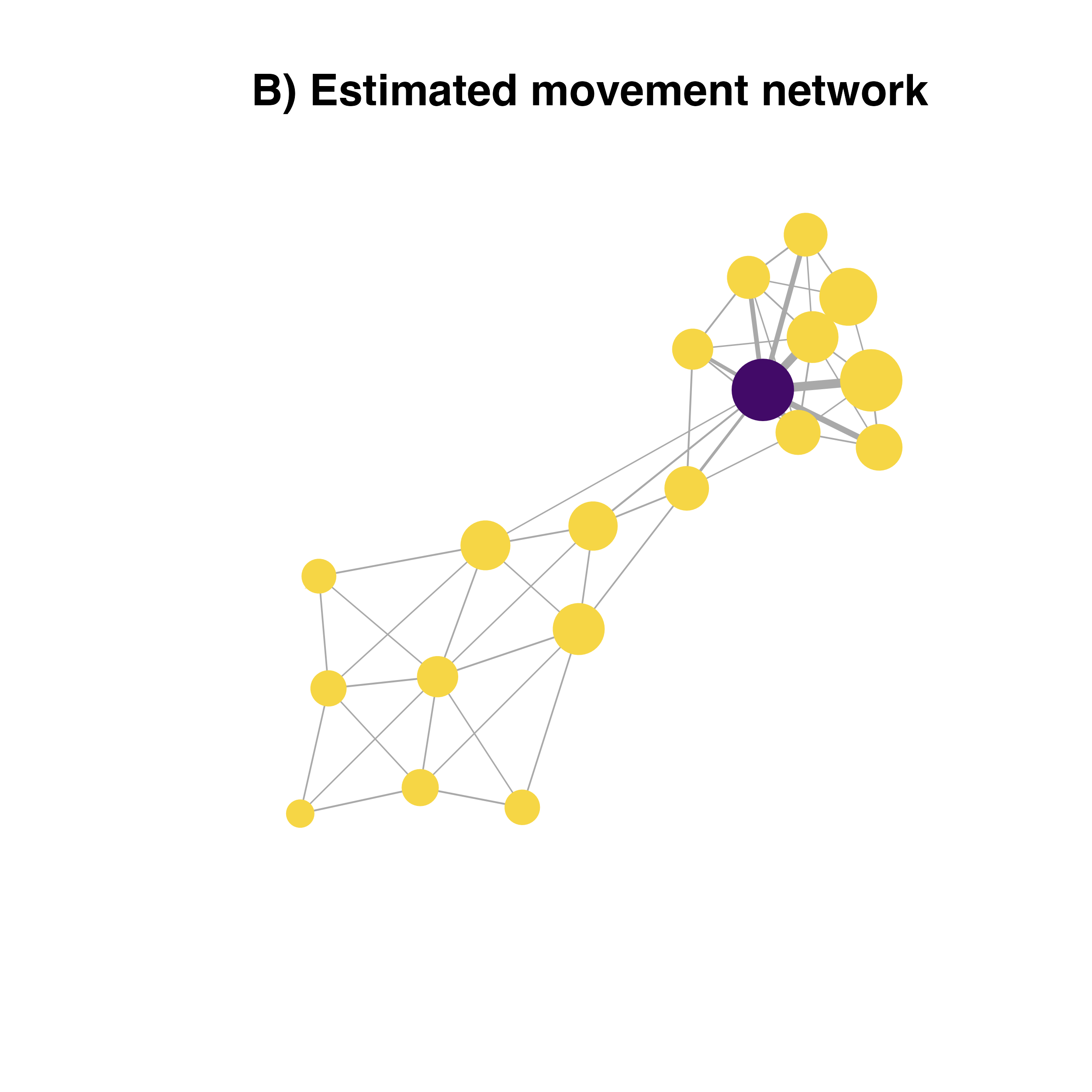

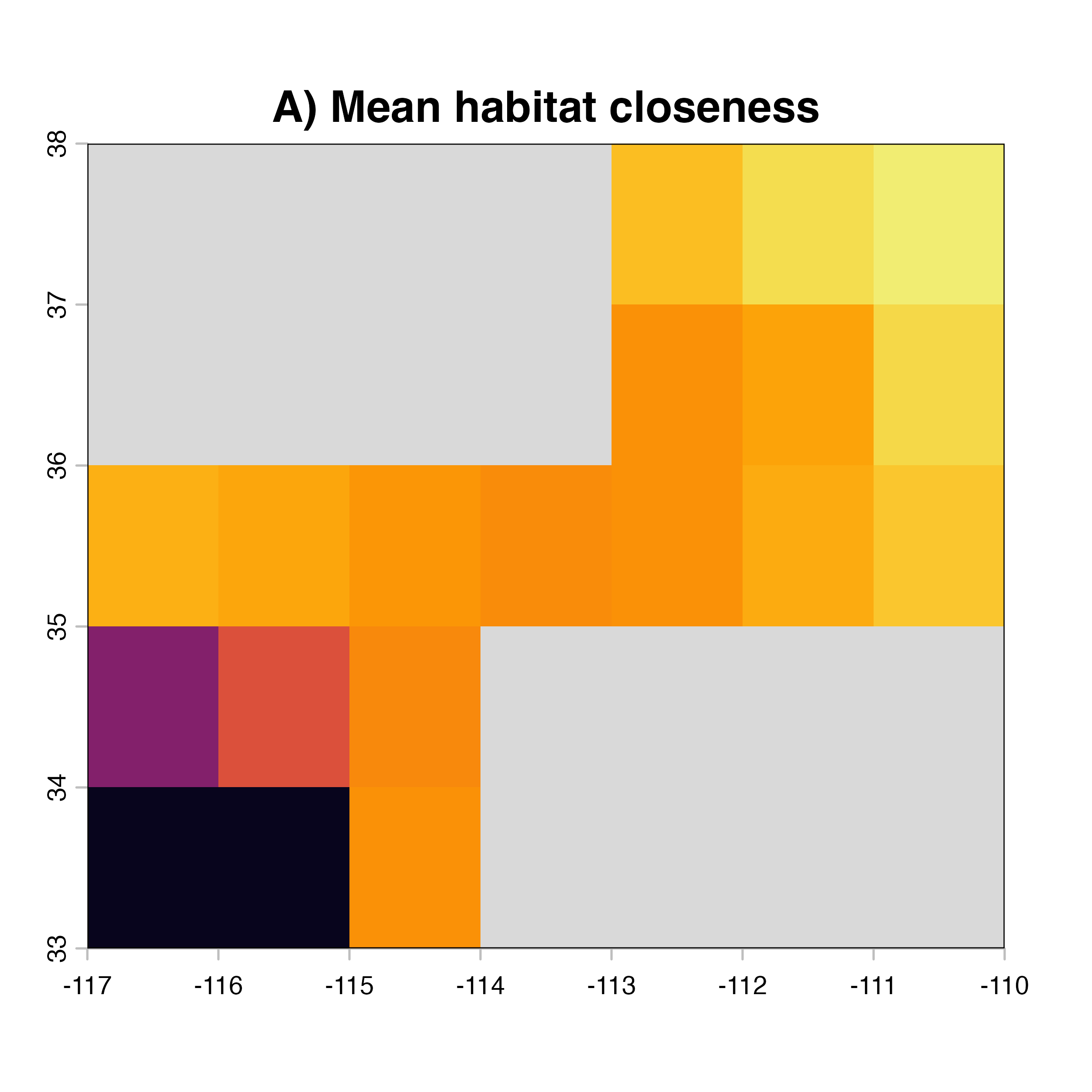
# plotting the map of surveillance priorities
xing.closeness<-xing.rast
values(xing.closeness)[nonZero]<-V(habitatnet)$closeness
plot(xing.closeness, col = vir.pal, colNA = "grey85",
     main = "C) Mean closeness centrality")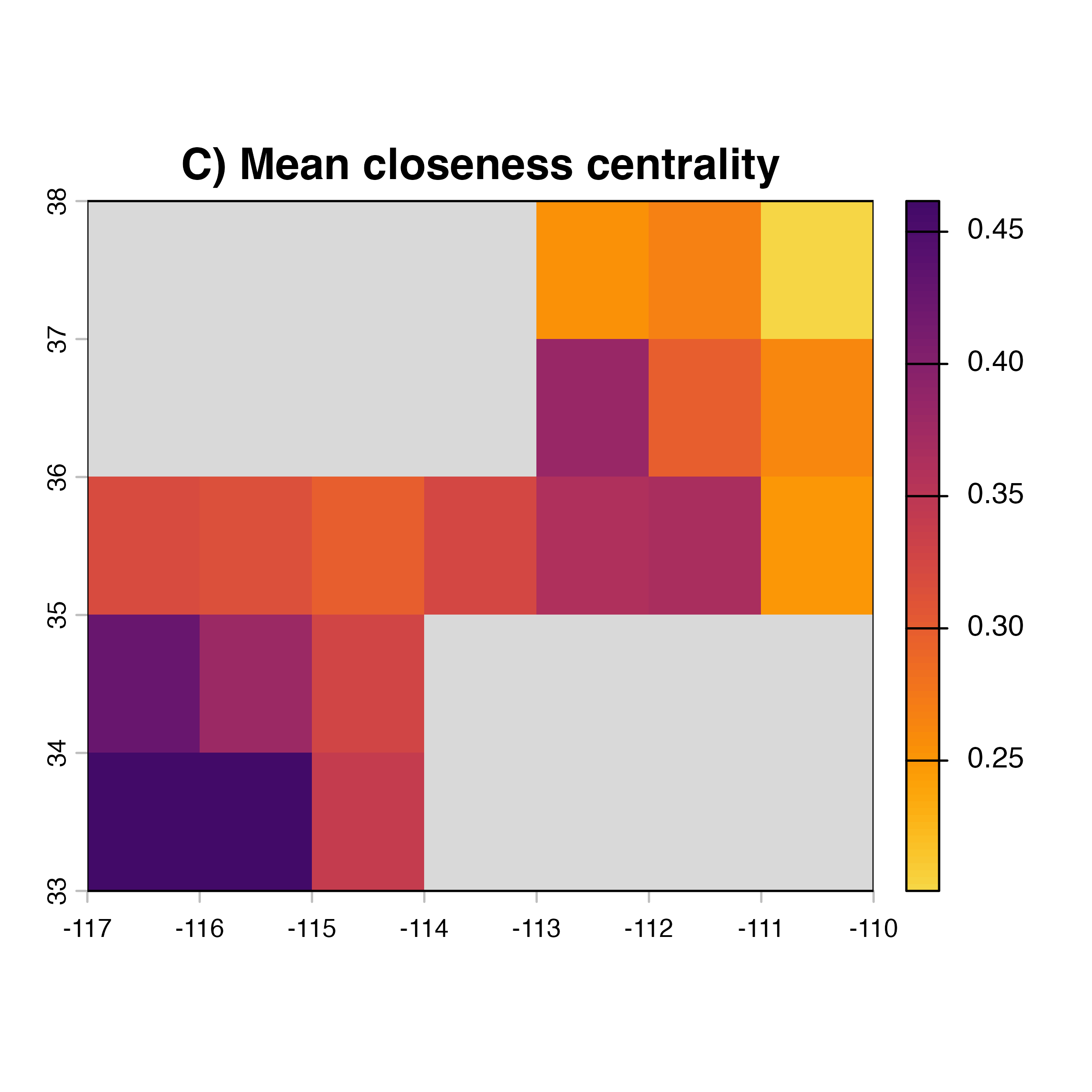

Illustrating the functionality of geohabnet

While you can conduct a habitat connectivity analysis running all lines of code provided above, geohabnet offers this functionality and more with a single function in R.

In our hypothetical example above from Xing et al 2020, you will only need to provide the SpatRaster object indicating the habitat density distribution to the msean function and specify all the parameters available in this function as you wish.

Lets first install the geohabnet package and then call the library in our environment. Then use the msean function to conduct a habitat connectivity analysis using the map of habitat density called xing.rast.

vir.pal<-viridis(n=100, option = "inferno", direction = -1, begin = 0.05, end = 0.95)
civ.pal<-viridis(80, option = "cividis", direction = -1, alpha = 0.95)
# Install the stable version of geohabnet package available in CRAN
# install.packages("geohabnet")

library(geohabnet)

## 
## Attaching package: 'geohabnet'

## The following objects are masked from 'package:igraph':
## 
##     closeness, degree

# Alternatively, you can install the development version from GitHub
# devtools::install_github("GarrettLab/HabitatConnectivity", subdir = "geohabnet")

# Using the habitat density map in geohabnet
net.metrics<-c("betweeness","closeness","node_strength","eigenvector_centrality","Sum_of_nearest_neighbors","page_rank")
net.label<-c("betweeness", "closeness", "node strength", "eigenvector centrality","nearest neighbors", "PageRank")
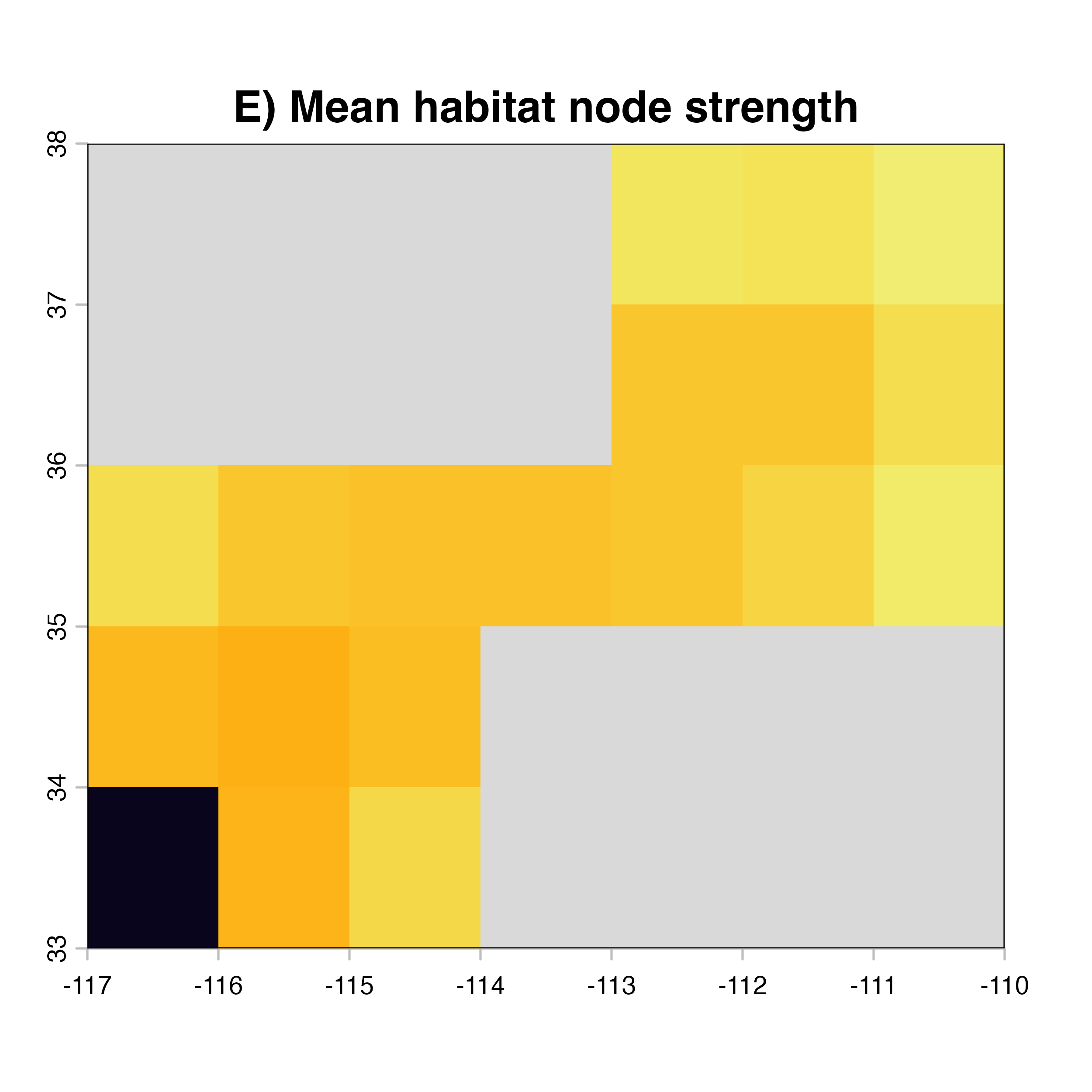
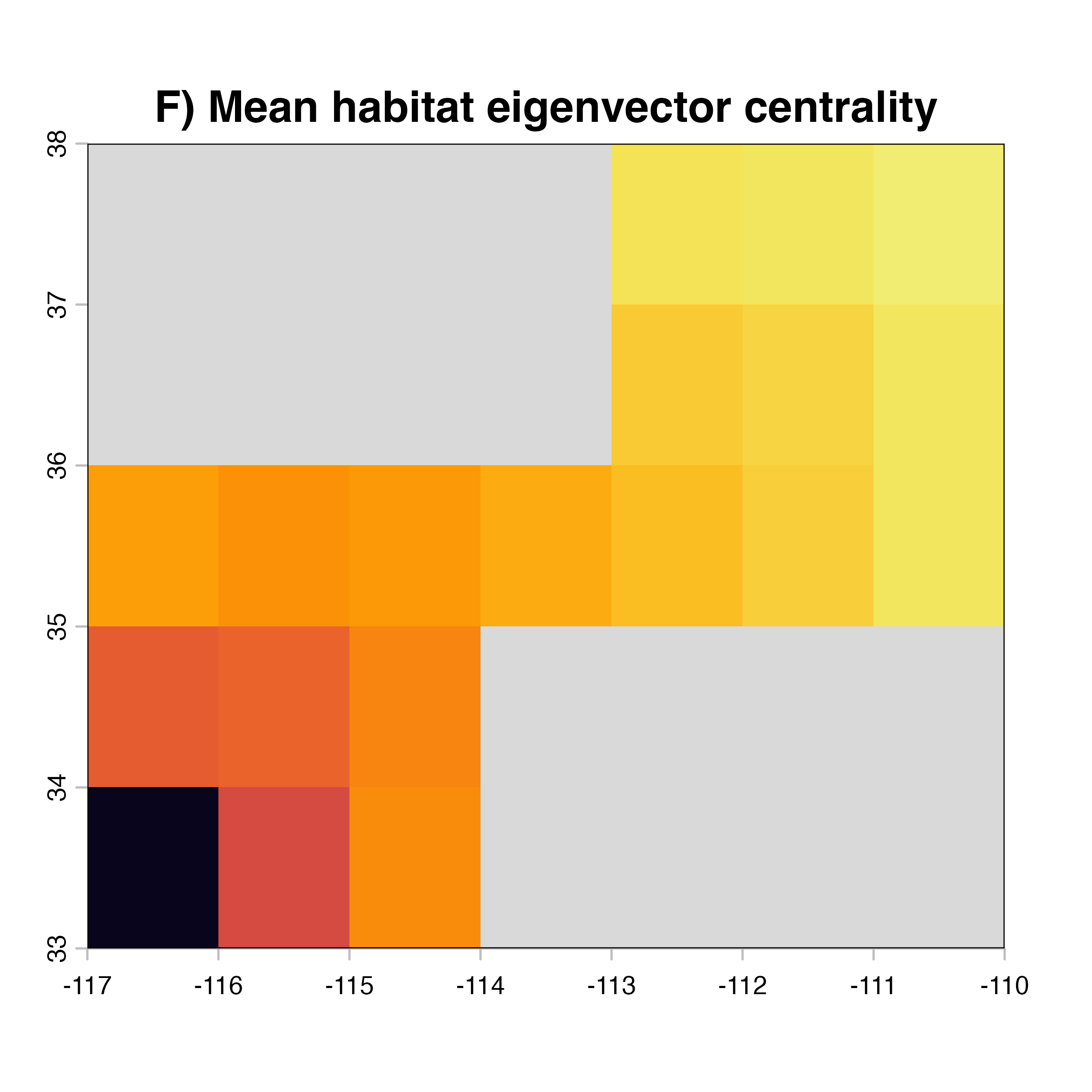
net.index<-c("D)","A)","E)","F)","G)","H)")

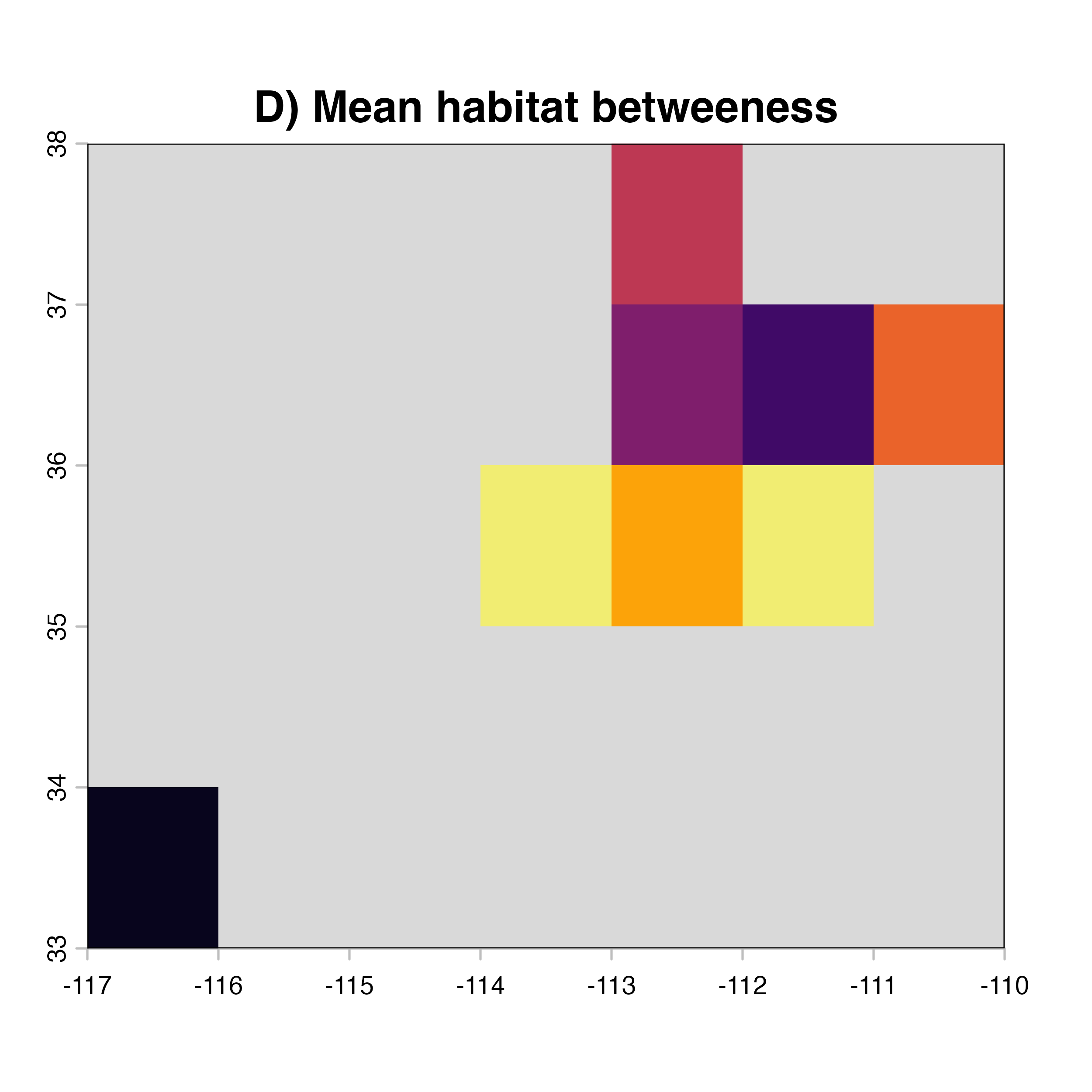
for (i in 1:4) {
  hab.net<-msean(xing.rast, res = 1, global = FALSE, maps = TRUE, 
               geoscale = c(-117,-110,32,38),link_threshold = 0.015,
               inv_pl = list(beta = c(0.25, 0.5, 0.7, 1, 1.5),
                             metrics = net.metrics[i], weights = c(100), 
                             cutoff = -1),
               neg_exp = list(gammas = c(0.05, 1, 0.2, 0.3),
                              metrics = net.metrics[i], weights = c(100),
                              cutoff = -1)
    )
   
  plot(hab.net@me_rast, col = vir.pal, legend = FALSE, colNA = "grey85",
     main = paste(net.index[i],"Mean habitat",net.label[i]))
  }

hab.net<-msean(xing.rast, res = 1, global = FALSE, 
               geoscale = c(-117,-110,32,38),link_threshold = 0.015,
               inv_pl = list(beta = c(0.25, 0.5, 0.7, 1, 1.5),
                             metrics = net.metrics[1:4], weights = c(50, 15, 15, 20), 
                             cutoff = -1),
               neg_exp = list(gammas = c(0.05, 1, 0.2, 0.3),
                              metrics = net.metrics[1:4], weights = c(50, 15, 15, 20),
                              cutoff = -1)
    )

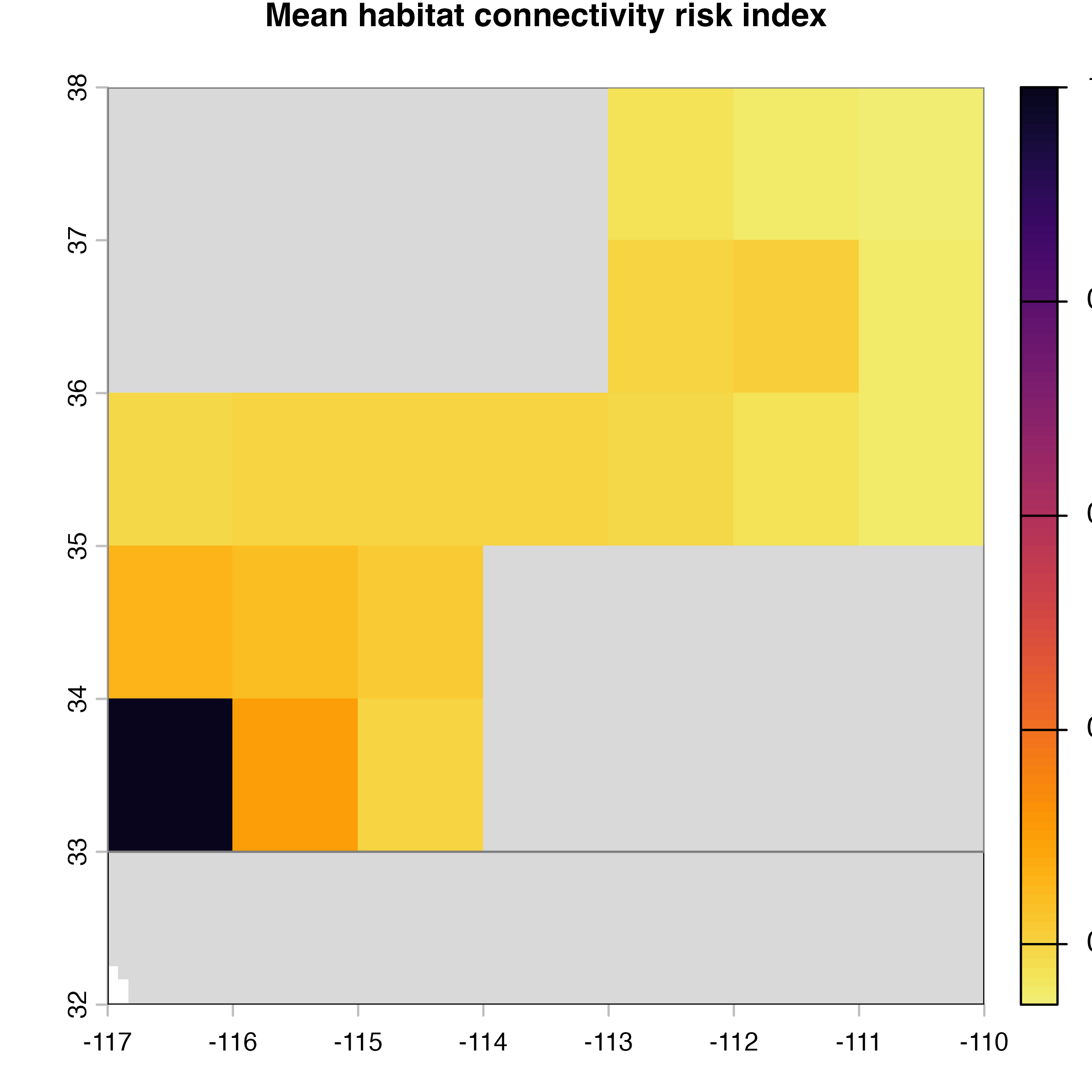
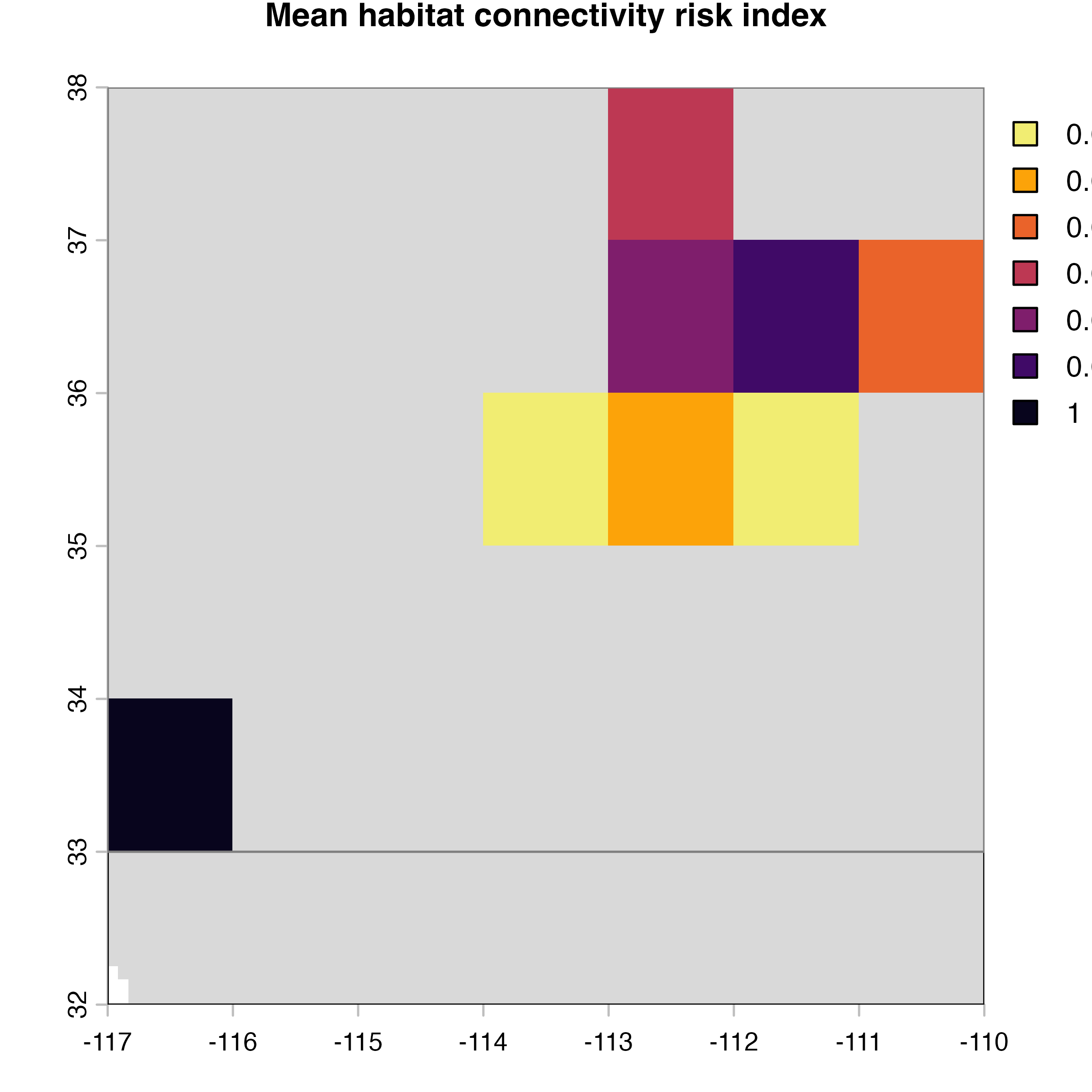
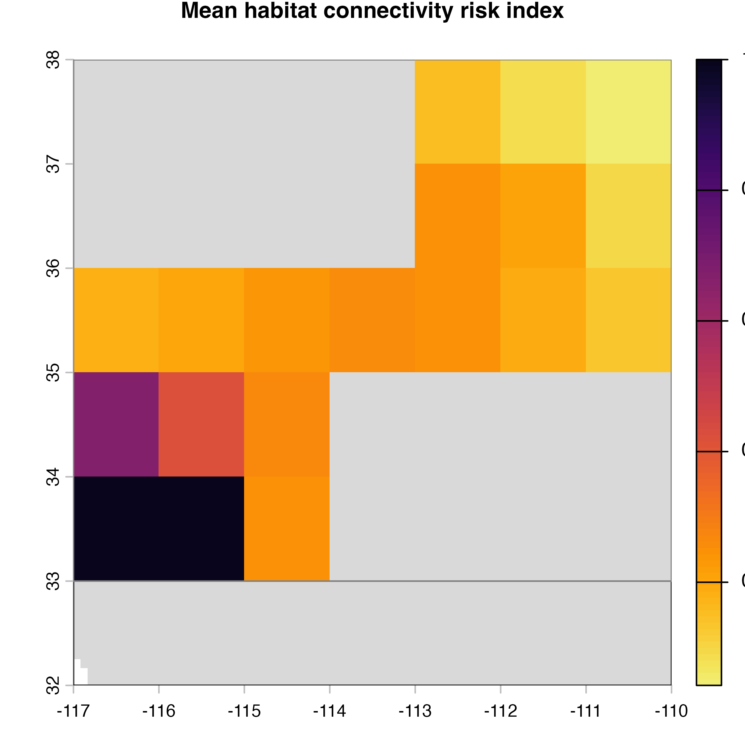
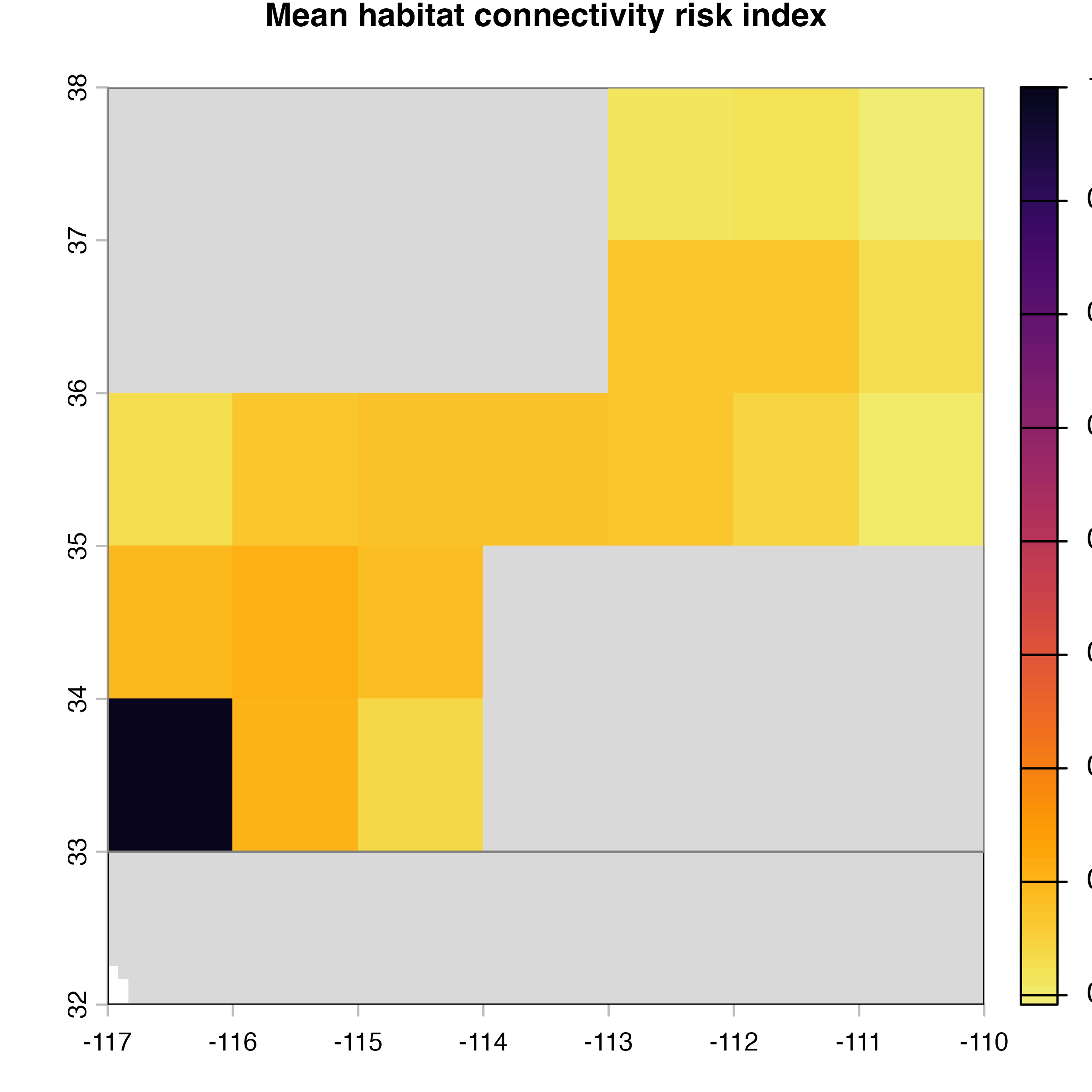
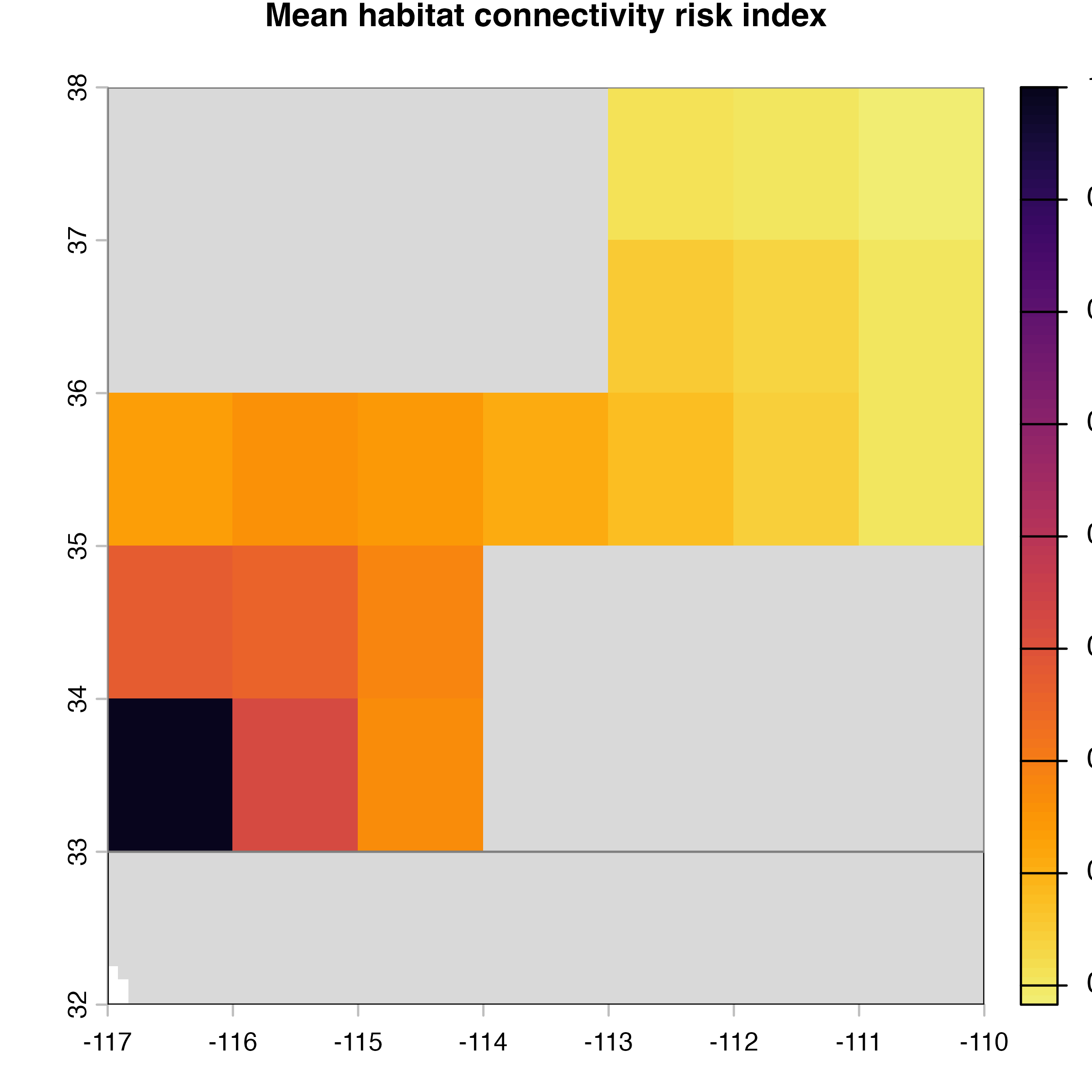
plot(hab.net@me_rast, col = vir.pal, colNA = "grey85",
     main = "G) Mean habitat connectivity index")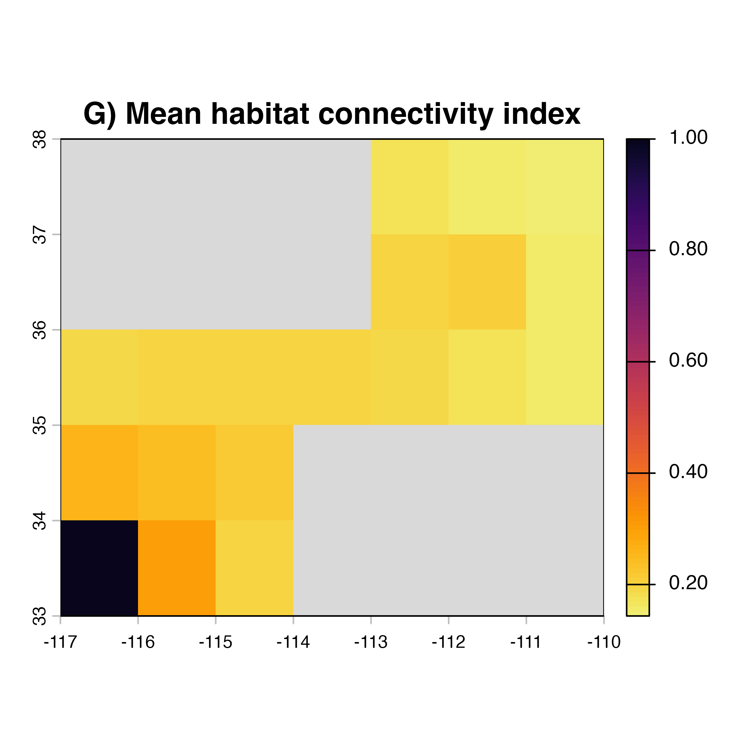

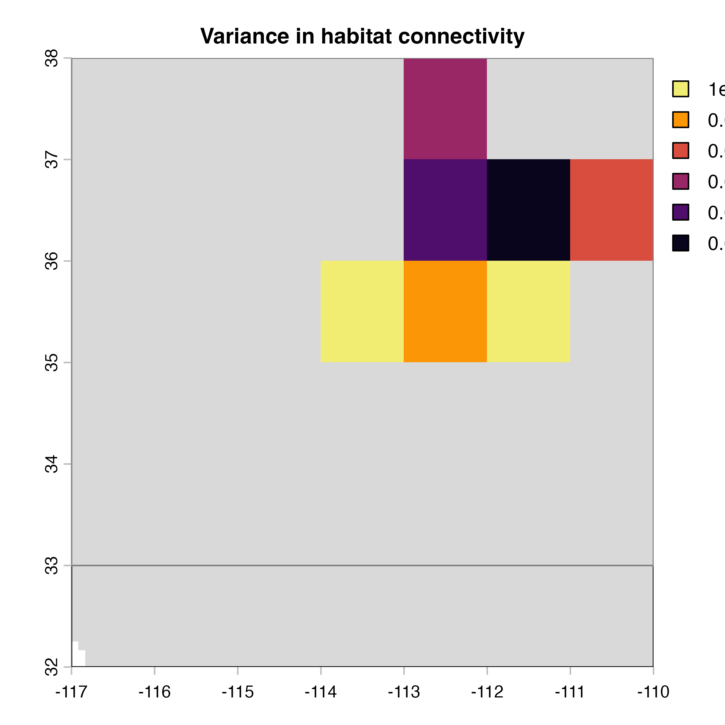
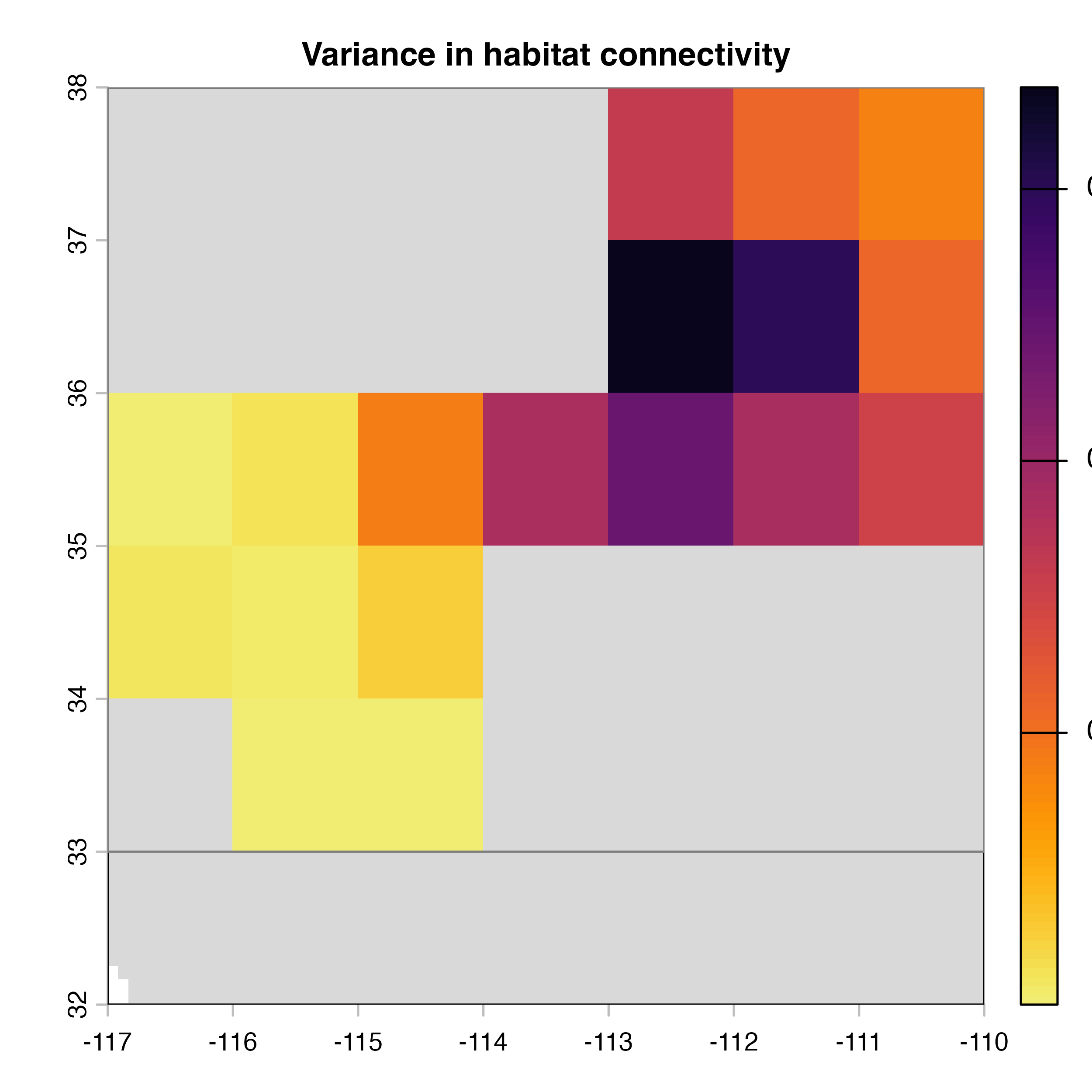
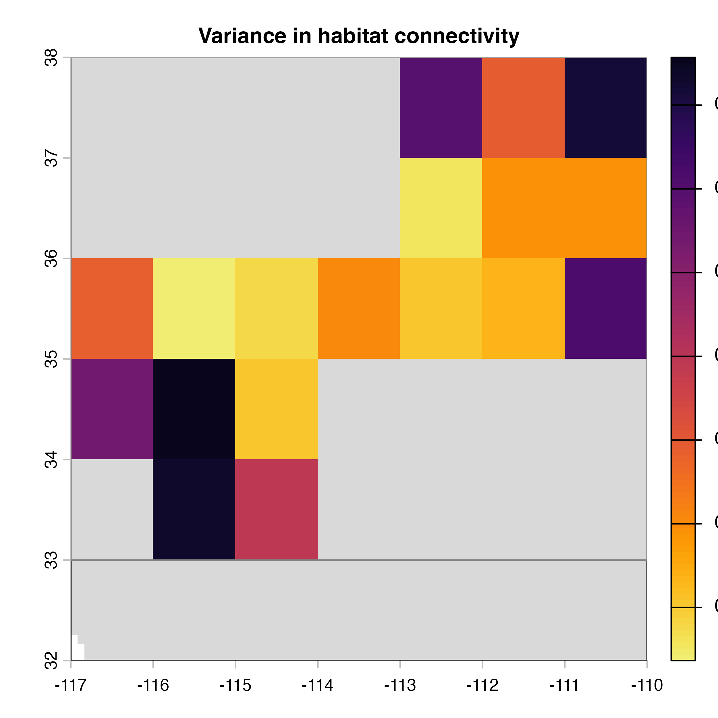
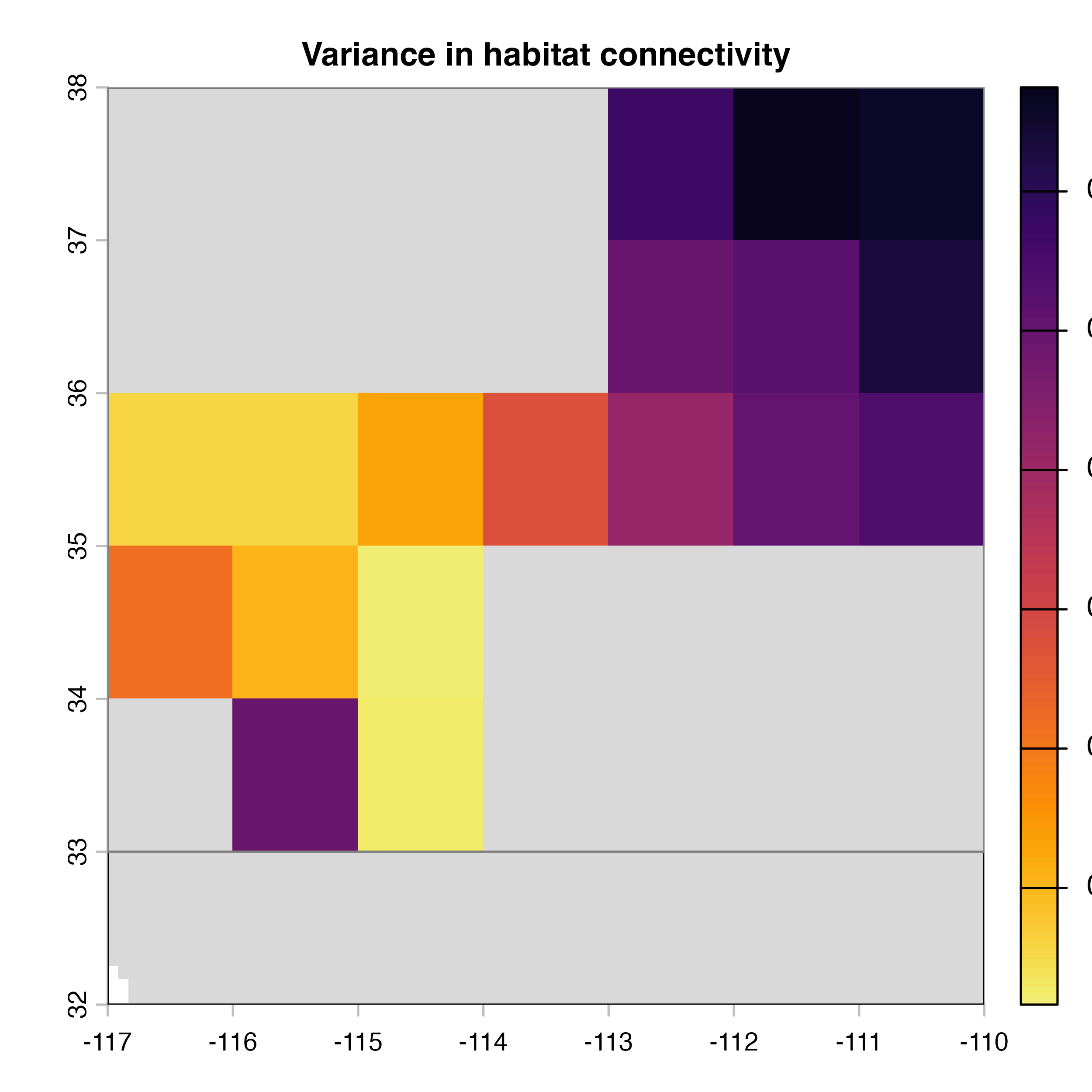
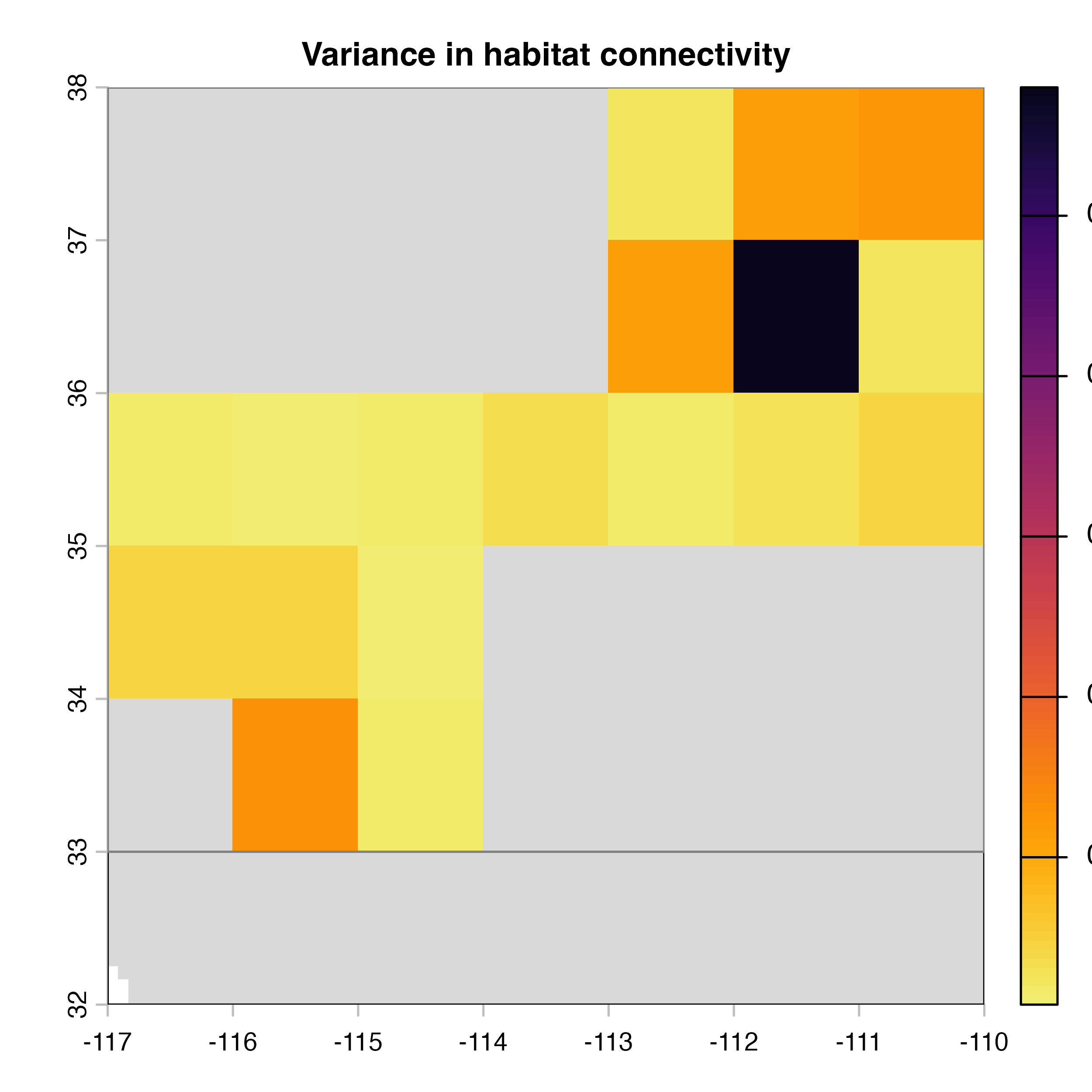
plot(hab.net@var_rast*100, col = vir.pal, colNA = "grey85",
     main = "H) Variance in habitat connectivity")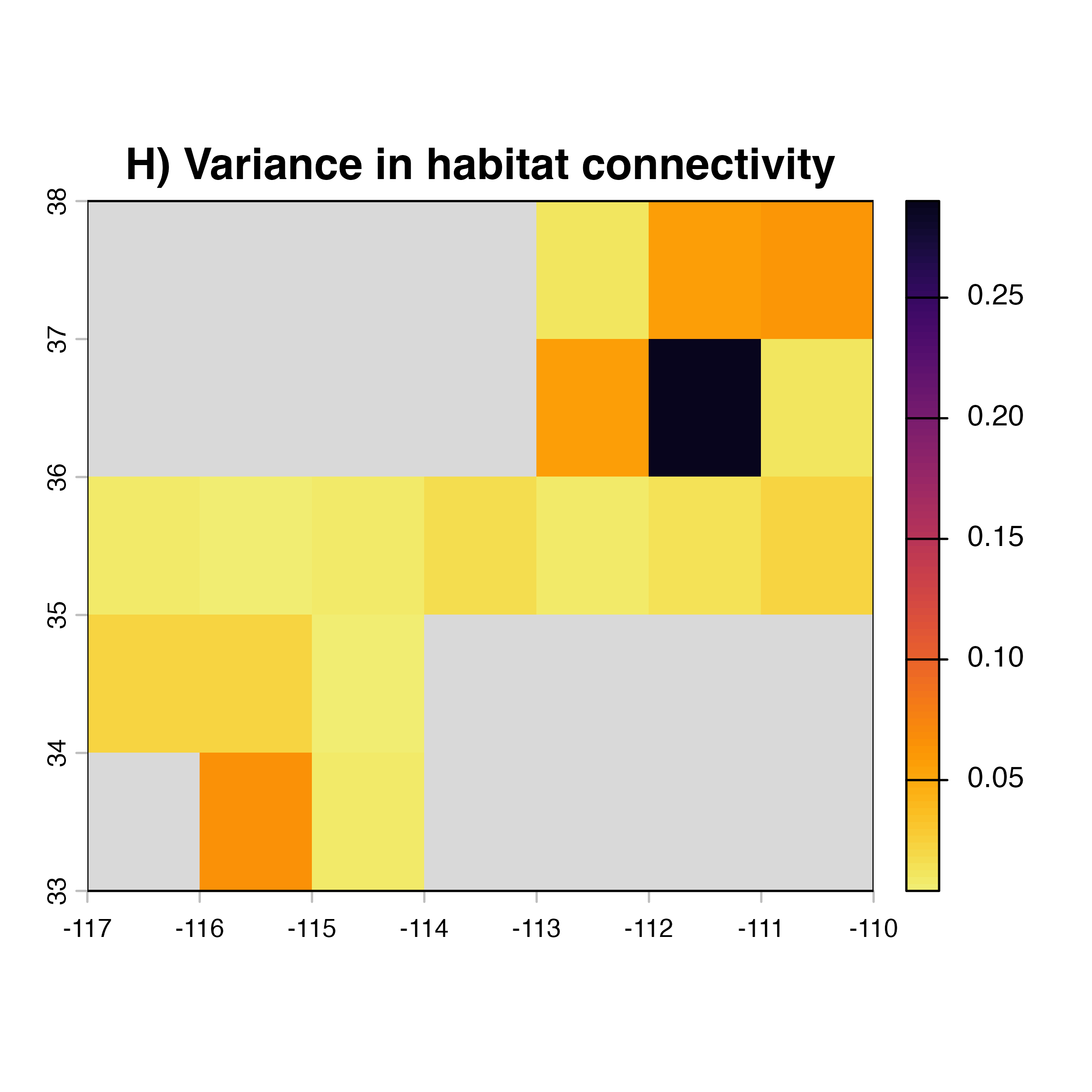

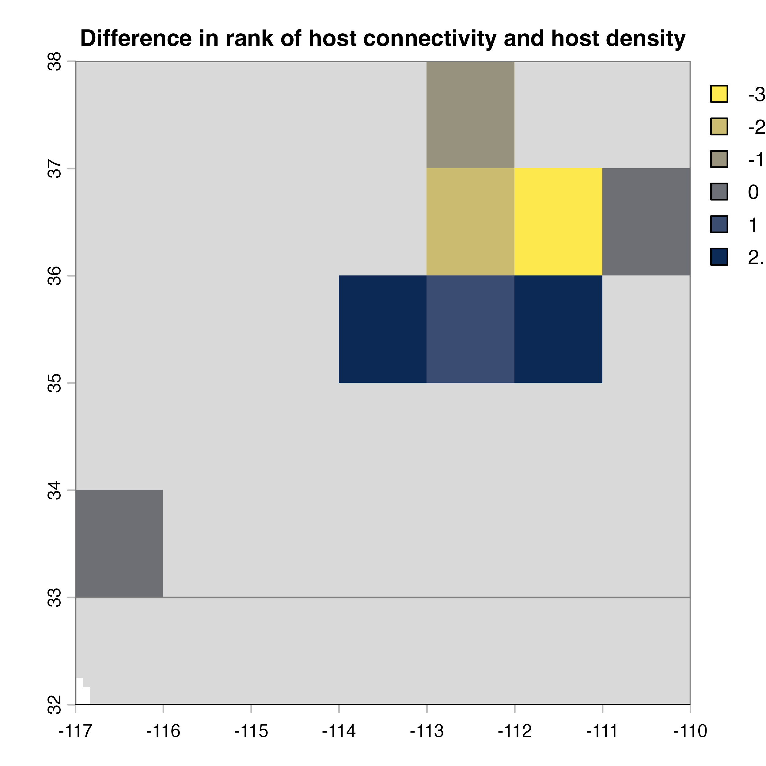
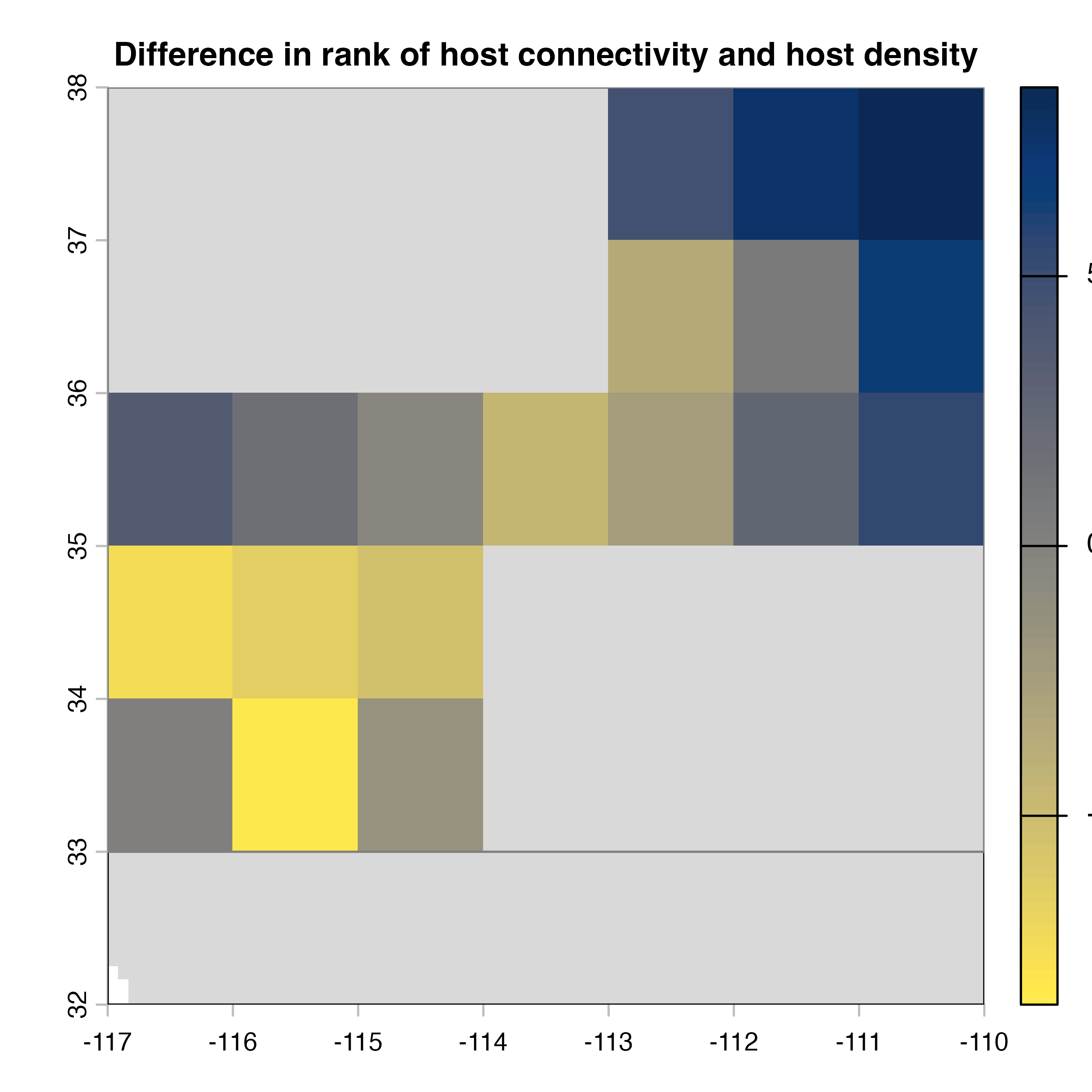
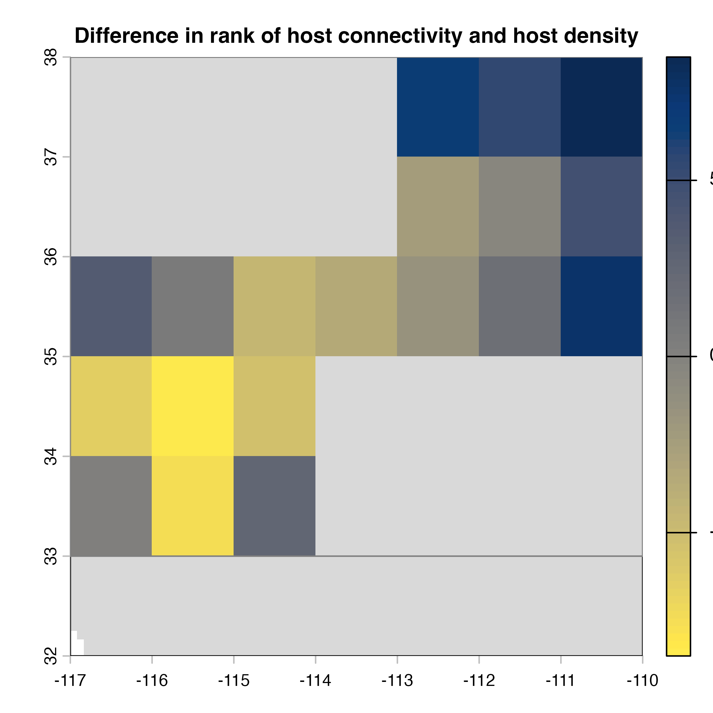
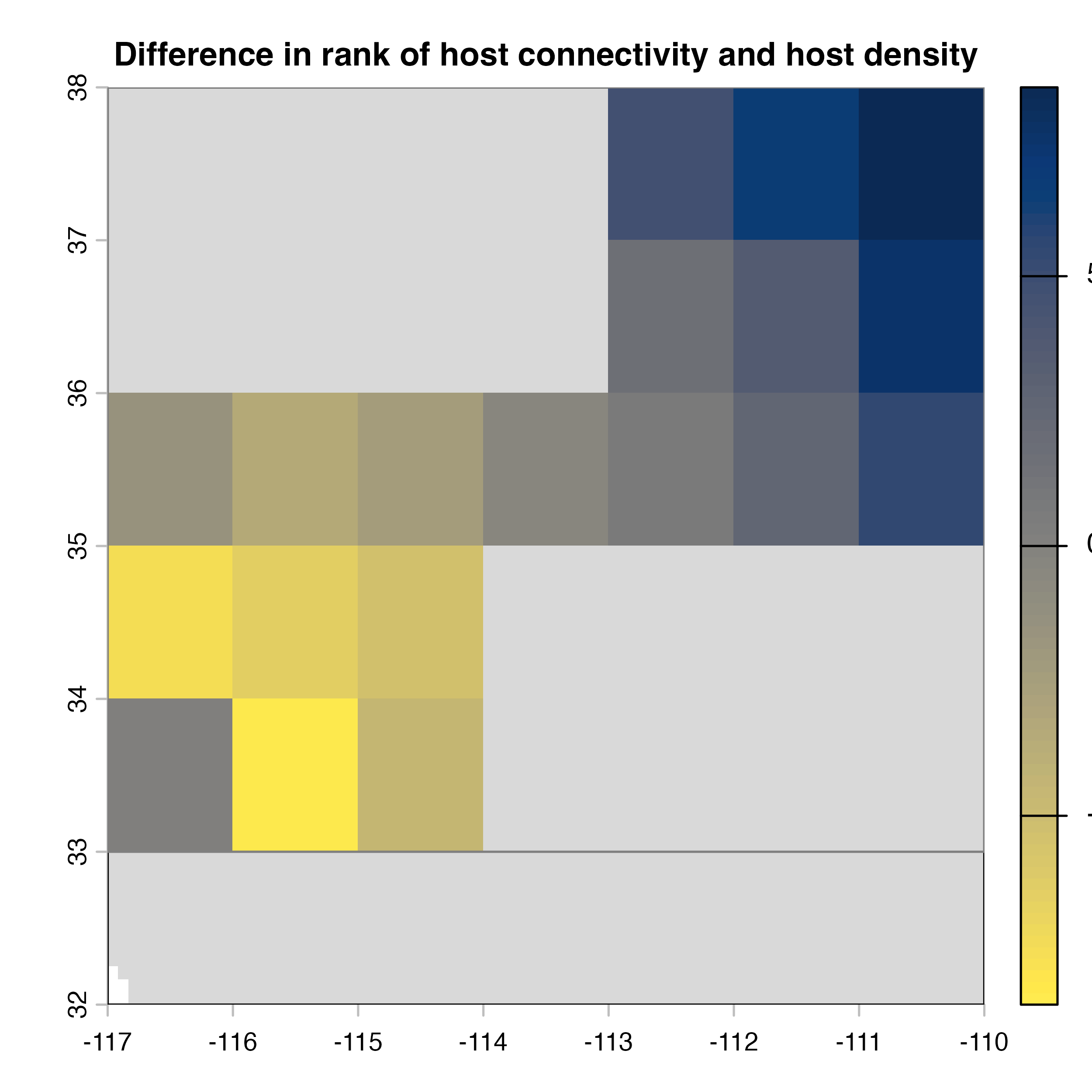
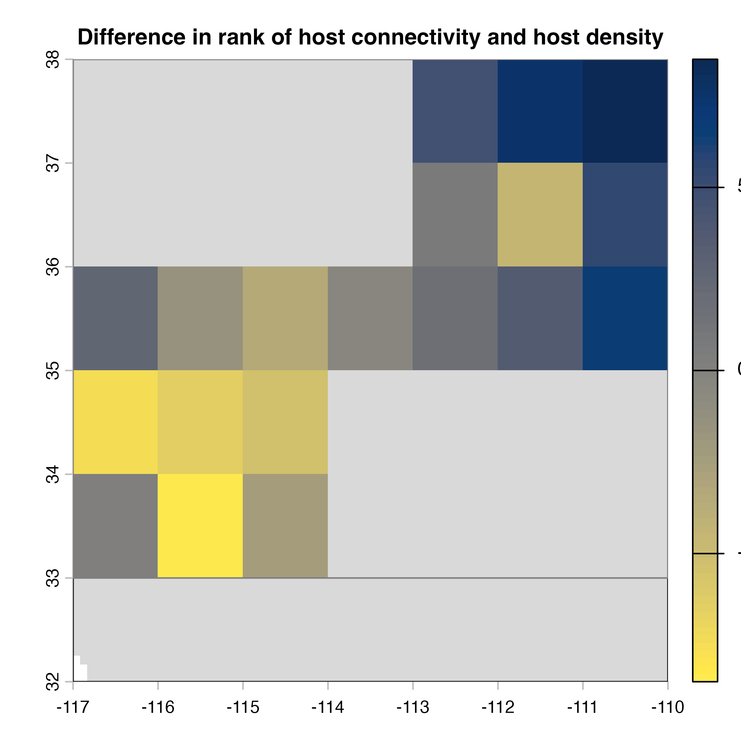
plot(hab.net@diff_rast, col = civ.pal, colNA = "grey85",
     main = "I) Mean connectivity - Habitat density")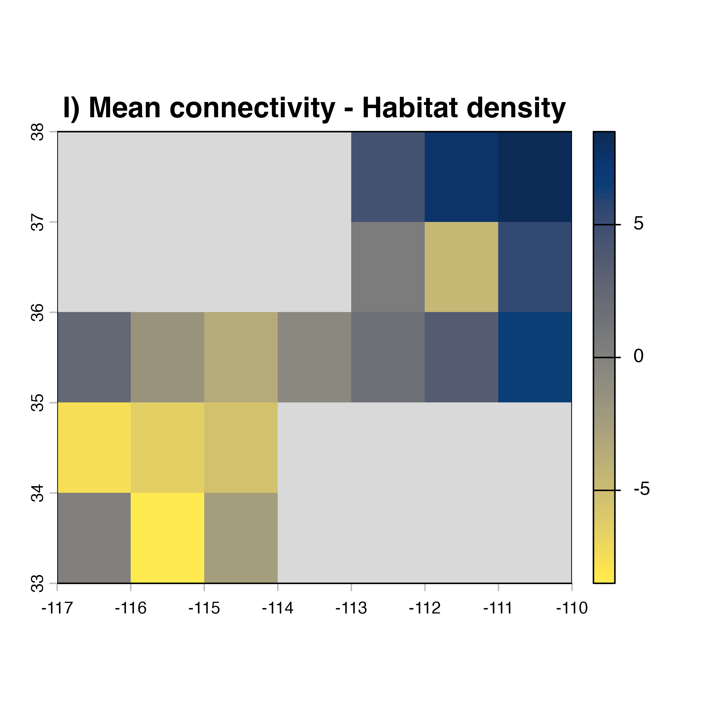

As you noticed, there are many parameters that can be modified in the msean function. This is because geohabnet is flexible so you can apply it to any pest or pathogen species. geohabnet takes all these parameters as inputs and conduct a sensitiviy analysis across these parameters to provide output maps. Play around with different parameter values and see what happens…

Note that in the code above, we explicitly extract the outputs (mean, variance and difference maps) from the object produced by geohabnet because Rmarkdown does not allowed us to directly plot these maps. :( But no worries: if you run msean in your console (not in the RMarkdown chunk), geohabnet will automatically get pictures of the three maps of habitat connectivity in the “Plots” panel in RStudio for you and do not have to deal with plotting.

A. I. Plex

11 June, 2026