User guide
Aaron Plex Sula (author)
plexaaron@ufl.eduKrishna Keshav (co-author)
krishnakeshav.pes@gmail.com11 June, 2026
Source:vignettes/articles/user_guide.Rmd
user_guide.RmdWelcome to the user guide for geohabnet (Plex Sulá 2025), an R package for the analysis of habitat landscape connectivity!
This section is designed for users already familiar with R and RStudio. While RStudio is considered an interactive environment, using R from the CLI is not. The pre-print for this application paper can be accessed here (Plex Sulá 2025).
The underlying theory for calculating habitat connectivity is based
on network analysis. To get an idea of the concepts of habitat
connectivity in geohabnet, users are recommended to check
(Xing et al. 2020) – Global cropland
connectivity: A risk factor for invasion and saturation by emerging
pathogens and pests. BioScience 70(9): 744-758.
Installation and pre-requisites
The geohabnet R package can be directly installed and
loaded in RStudio using the following commands. For the stable version
published in CRAN:
install.packages("geohabnet")This version 2.2 is available in CRAN
For the latest development version available on GitHub:
install.packages("devtools")
devtools::install_github("GarrettLab/CroplandConnectivity", subdir = "geohabnet")
This version is available at the GitHub repository
In either case, the user will be prompted to update dependencies to
other R packages during the installation in RStudio. We recommend
updating all the package dependencies. The dependencies of the
geohabnet package and their minimum versions required can
be accessed by the following code:
desc::desc(package = "geohabnet")Note that desc::desc() is a function from an external
package and requires installation for its use. Now, the geohabnet (Plex Sulá 2025) package can be loaded into the
current R environment.
Getting started
The landing page and documentation can be accessed using
?geohabnet. This guide was written for geohabnet 2.2, which
is available for download in CRAN and GitHub.
The help page for all the functions can be accessed with
?geohabnet::fun or help(geohabnet::fun), where
fun needs to be changed to the name of a function of your interest. For
example, ?geohabnet::msean() or simply ?msean
will provide documentation for the function msean().
geohabnet 2.2 provides two main functions to estimate
and map the connectivity of locations where habitat is present
(hereafter, habitat connectivity): sensitivity_analysis()
and msean(). The package also offers supplementary
functions, but they are not covered in this user guide. Before running
the function, please review the description of each parameter below.
Well, there are over ten parameters that can be used in either
sensitivity_analysis() or msean(). The
parameters in msean() can be modified directly within the
function in RStudio, as is common in many R packages.
sensitivity_analysis() requires a list of parameters,
providing an organized way to easily change the default parameter values
without listing them every time. The list of parameters for
sensitivity_analysis() is called
parameters.yaml.
The following steps allow you to access the parameters.yaml
file, specify parameter values, and use them for analysis in
sensitivity_analysis():
- You can get the parameters.yaml file by running
geohabnet::get_parameters()and specifying the location where the file will be saved. Useiwindow = TRUEfor interactive selection or provide an absolute file path to the parameter out_path for non-interactive use. For example, Plex ran the following:
get_parameters(out_path = "C:/Users/plexaaron/Documents")Open the parameters.yaml file in any program that allows you to edit it (outside RStudio). Please do not alter the structure of the yaml file and parameter names to ensure it will be successfully compatible with
sensitivity_analysis(). Except for host, this file will contain default acceptable values for the supported parameters (see picture below).Manually modify or add values in the parameters.yaml file and save it.
Feed the new parameters.yaml file to the package using
geohabnet::set_parameters()which will return TRUE if the parameters were set successfully. For example, Plex ran the following:
set_parameters(new_params = "C:/Users/plexaaron/Documents/*parameters.yaml")- Now you can run
sensitivity_analysis()to produce maps of habitat connectivity.
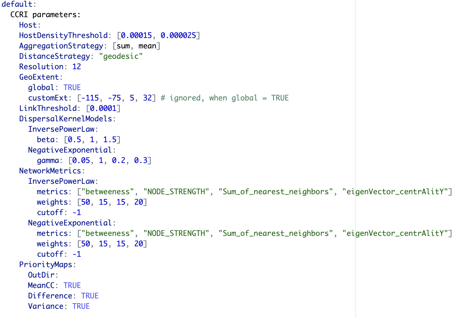
Figure 1. Initial parameter values in the
parameters.yaml file for
sensitivity_analysis().
Setting parameters in sensitivity_analysis() and msean()
1. Providing habitat distribution
Users can provide any type of habitat map that is compatible with the
terra:rast() function. Typically, this is a TIFF file in
the standard geographic coordinate system (WGS84). Acceptable entries in
this SpatRaster range from zero (no habitat is available in a location)
to one (the location is fully covered with habitat for a species).
Host availability is an important component of habitat quality for
plant pathogens. Here, we provide two ways for providing maps of host
availability for geohabnet. The first one is indented for
using your data, and the latter is based on data sources for the global
distribution of crop hosts.
-
Your own data. The
geohabnetpackage is designed to accept raster files as inputs for the distribution of habitat availability. You can provide your raster file in two ways:
To use sensitivity_analysis(), you can specify the
absolute path or location of your raster file in the
Parameters.yaml under Host (see example in the
figure above).
To use msean(), the user is required to read the habitat
map directly in R. For example:
hab.rast <- terra::rast("habitat-map-example.tif")- Monfreda Dataset. Monfreda et al. (2008) provides information for the geographic distribution of 172 crop categories. These maps can be used as a first approximation for the habitat quality of plant pests.
You can access this dataset directly in R using the
geodata package. Run geodata::monfredaCrops()
in your console to check which crops are available in the Monfreda
dataset. You can use a SpatRaster of the crop of interest in
geohabnet with the following code:
library(geodata)
hab.rast <- crop_monfreda(crop = "banana", var = "area_f", path = tempdir())
library(geohabnet)
msean(rast = hab.rast)
Alternatively, you can access the Monfreda dataset by downloading
crop distribution maps from EarthStat. You can then provide the
location of the downloaded TIFF file in the parameters.yaml
file when using sensitivity_analysis().Note that an updated
version of the Monfreda dataset is the [CROPGRIDS dataset] (https://doi.org/10.6084/m9.figshare.22491997), though
data layers need to be transformed from harvested area to cropland
fraction.
-
MAPSPAM dataset. This dataset provides information
for the global distribution of 42 crops or crop groups (IFPRI 2019). You
may want to use the harvested area or physical area for your analysis of
habitat connectivity in
geohabnet: You can access this dataset in R using thegeodatapackage. Rungeodata::spamCrops()in your console to check which crops are available in the MAPSPAM dataset. You can use a SpatRaster of the crop of interest ingeohabnetwith the following code:
library(geodata)
library(terra)
hab.rast <- crop_spam(crop = "banana", var = "phys_area", path = tempdir())
conv.factor <- res(hab.rast)[1]*111000 * res(hab.rast)[1]*111000 / 10000
hab.rast <- hab.rast$banana_phys_area_all / conv.factor
library(geohabnet)
msean(rast = hab.rast, res = 24)
Note that we convert the physical area of crop availability in
hectares to the fraction of total area occupied by the crop. The
conv.factor estimates the total area of each grid cell in
hectares.
Alternatively, you can access the MAPSPAM dataset by downloading crop
distribution maps from MAPSPAM.
Note that newer versions of MAPSPAM are not available in the
geodata package, as of October 10, 2025.
- You may prefer that your analysis be based on both the Monfreda and MAPSPAM datasets. In this case, you may first get a spatRaster with host density for the target crop category from each dataset and then average them to generate a SpatRaster of the mean host availability. Another situation is that you need to add different crop categories into a SpatRaster because the habitat of a species ranges across multiple crop species.
2. Selecting habitat threshold
Now that you have selected the habitat landscape for your analysis, the next step is to set a threshold for habitat availability. The habitat threshold is the minimum proportion of habitat available in the grid cells (or locations) that will be included in the analysis. Choosing a habitat threshold is useful when the user needs to focus the connectivity analysis on more important locations in the landscape, reducing the computational expense needed to run the analysis. Likewise, some species might require an minimum level of habitat availability for movement.
In geohabnet, this parameter is called
HabitatThreshold and can support any values between 0 and
1. Note that a sensitivity analysis can be conducted by specifying a
list of values for the habitat threshold. To prevent errors, ensure that
the values for the habitat threshold are less than the maximum value of
habitat availability on the map you provided.
3. Selecting a spatial aggregation strategy
Aggregation strategy refers to the function used to create a new map of habitat availability with a lower resolution (larger cells). Reducing the spatial resolution reduces the computational power needed to run the habitat connectivity analysis. It also helps evaluate how habitat connectivity changes from fine to coarse resolution.
In geohabnet, there are two aggregation strategies:
If
AggregationStrategy: [sum], then the sum of the habitat availability of a set of small grid cells is divided by the total number of small cells within the resulting larger grid.If
AggregationStrategy: [mean], then the sum of the habitat availability of a set of small grid cells is divided by the number of small cells containing only land within the large grid. In this strategy, small cells with water are excluded from spatial aggregation.
4. Selecting spatial resolution
In geohabnet, the aggregation factor or granularity is
the number of small grid cells used to generate or aggregate into a
larger grid cell (horizontally and vertically). For example, the finest
spatial resolution of the MAPSPAM and Monfreda datasets is 5 minutes,
and a granularity value of 6 will result in maps with a spatial
resolution of 0.5 degrees. Table 1 compares the spatial resolution and
sizes of grid cells for different values of granularity that can be used
to aggregate the maps from the MAPSPAM or Monfreda.
Table 1. Spatial resolutions and their corresponding granularity.
| Spatial resolution (degree) | Spatial resolution (minutes) | Grid size (km²) | Grid area (km²) | Granularity |
|---|---|---|---|---|
| 1° | 60 mins × 60 mins | 111 × 111 km² | 12,394 km² | 12 |
| 0.5° | 30 mins × 30 mins | 55.7 × 55.7 km² | 3,102 km² | 6 |
| 0.25° | 15 mins × 15 mins | 27.8 × 27.8 km² | 772 km² | 3 |
| 0.1667° | 10 mins × 10 mins | 18.5 × 18.5 km² | 342 km² | 2 |
| 0.0833° | 5 mins × 5 mins | 9.27 × 9.27 km² | 85 km² | 1 |
You can choose the spatial resolution of the analysis using the
Resolution parameter, which currently supports a single
integer value of 1 or greater.
If you want to check which spatial resolution is being used in the analysis, run
reso()in the console.Setting the spatial resolution directly in parameters.yaml file is recommended.
Analysis at finer (higher) spatial resolution can be more computationally expensive. For example, using a 6 CPU machine, a global analysis of host connectivity at one-degree resolution for coffee croplands can last 20-30 minutes, and for wheat croplands, more than two hours.
6. Selecting geographic extent
The geographic extent refers to the rectangular area for analysis
where there is (obviously) at least one grid cell with a habitat
available. The geographic extent must be specified with four values
representing the geographic limits of the area for analysis, following
the order: minimum longitude, maximum longitude, minimum latitude, and
maximum latitude. The geographic extent in geohabnet is
specified in degrees, which are in decimal notation and have a negative
sign for the southern and western hemispheres.
In Parameters.yaml, two options are available to set the
geographic extent of the analysis with the parameter
GeoExtent.
-
If you want to execute your analysis on a global extent, then you set
global: TRUE.- If you want to check what the global extent coordinates are, run
global_scales()in the console. - If you want to change the default coordinates of the global extent,
you can use the function
set_global_scales(). - The default coordinates for the global geographical extent cannot be set using the parameters.yaml.
- If you want to check what the global extent coordinates are, run
If you want to run an analysis where the geographic extent is a continent, a country, or any other geographic extent smaller than a continent, then you can use the option
customExtunderGeoExtent. Please do not forget to setglobal: FALSE. Otherwise, ifglobal = TRUE, thencustomExtis ignored.
7. Selecting a dispersal kernel model
In geohabnet, two dispersal kernel models are used to
calculate the “relative likelihood” of species movement between
locations. These dispersal kernels are also commonly used in movement
ecology.
In Parameters.yaml, set any of the following options under
DispersalKernelModels:
- If you are interested in the inverse power law model, then set the dispersal parameter beta to any positive decimal value.
- If you are interested in the negative exponential model, then set the dispersal parameter gamma to any positive decimal value.
- You can use both dispersal kernel models and evaluate multiple dispersal parameter values in each model simultaneously in the analysis.
Now you may be wondering or panicking about two questions. No worries, we gotcha.
First, which dispersal kernel model should I use? Tough question… Table 2 provides some characteristics for each dispersal kernel that can help you decide which one to use in the analysis.
-
Second, which values for the dispersal parameters beta and gamma are best? Another tough question… (hahaha) Figure 2 provides an estimation of the dispersal parameters beta and gamma for a variety of plant pests, which can help answer this question:
Smaller dispersal parameter values result in higher probabilities of species dispersal.
The mean parameter beta is 1.72.
The mean parameter gamma is 0.345.
Table 2. Characteristics of the two common dispersal kernels for range expansion of species, after (Brown and Hovmøller 2002).
| Characteristic | Negative exponential model | Inverse power-law model |
|---|---|---|
| Model | exp(–γ × distance) | distance^–β |
| Dispersal parameter | Gamma | Beta |
| The tail of probability distribution | The dispersal probability distribution “tail” is exponentially bounded. Thus, long-distance dispersal events will be assigned a very low probability of occurrence. | The dispersal probability distribution is “fat-tailed.” Thus, very long-distance dispersal events are assigned a higher probability compared to the negative exponential model. |
| Rate of epidemic front | Constant | Accelerating, relative to the initial inoculum |
| Range expansion of the epidemic | Steady | Accelerating |
In conclusion, the inverse power law model is often useful to model long-range spread of a species, while the negative exponential model is more useful to assess short-range spread.
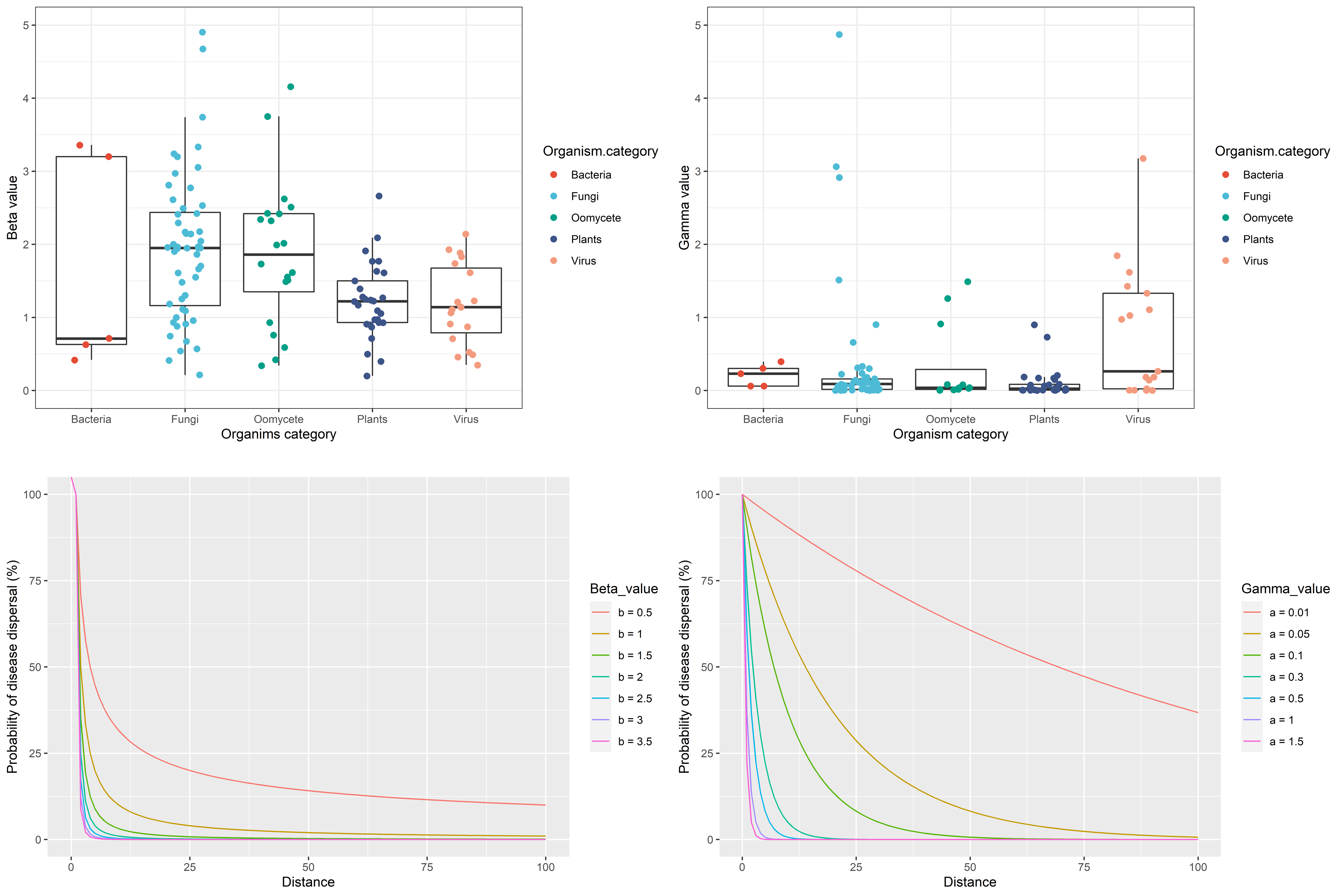
Figure 2. Beta values estimated from empirical studies (5 bacteria, 47 fungi, 20 oomycete, 29 plants, and 19 viruses) for inverse power law models (top left panel). Comparison of different beta values on the expected disease dispersal along ‘free-scale’ distance (top right panel). Gamma values estimated from empirical studies for negative exponential models (bottom left panel). Comparison of different gamma values on the expected disease dispersal along ‘free-scale’ distance (bottom right panel). Over 127 observations, most parameter values β are in a range of 0.5 and 3.5, mean 1.72, variance 1.25, and mode 0.93. Most parameter values γ are in a range of 0.01 and 0.5, mean 0.345, variance 0.55, and mode 0.015 or 0.06.
8. Selecting link weight threshold
Based on the information on habitat distribution and dispersal kernels, adjacency matrices are created, where entries represent the potential of species movement between habitat locations. Then, adjacency matrices are converted into graph objects to perform a network analysis, where the entries in the adjacency matrices are now the weights of the links of the network.
Choosing link weight thresholds helps to focus the analysis on the more likely species dispersal in the landscape.
Just like what you did with the habitat threshold, you can provide a
list of positive values to LinkThreshold in the
parameters.yaml file. Before running the
sensitivity_analysis() function, please check that the
values for the link weight threshold are smaller than the maximum link
weight in the network to prevent errors.
9. Selecting network metrics
In network analysis, there are different perspectives on how to determine which locations in the landscape are relatively more important. In the initial framework proposed by Xing et al. (2020), the cropland connectivity risk index included four different network metrics to evaluate the importance of locations in the landscape.
The geohabnet package provides the flexibility for the
user to choose among seven different network metrics to calculate the
connectivity of locations (Table 3) and to choose how each network
metric is weighted in the analysis. You can run the
supported_metrics() function in the console to check which
network metrics are supported by geohabnet.
Table 3. Network metrics that are available in the
geohabnet package.
| Network metric | Function in geohabnet
|
Rationale |
|---|---|---|
| Betweenness | betweeness(crop_dm, we) |
Betweenness centrality emphasizes the importance of a node acting as a bridge by connecting parts of the network that would otherwise be separate. Paths with more weighted links (that is, “shortest paths”) imply faster species movement between different regions of the network. |
| Node strength | node_strength(crop_dm, we) |
Node strength measures the sum of the link weights of a location. ADD INTERPRETATION |
| Sum of nearest neighbors | nn_sum(crop_dm, we) |
ADD DEFINITION — ADD INTERPRETATION |
| Eigenvector centrality | ev(crop_dm, we) |
Eigenvector centrality measures how locations having many neighbors’ neighbors through long paths in the network can facilitate the flow of pathogen spread. A location in a network can be important, by this measure, because it connects to lots of locations (even though those locations may be less important in risking themselves) or connects to a few locations at high risk. |
| Closeness | closeness(crop_dm, we) |
Closeness centrality indicates (i) the relative importance that the spread of a species in a node can access or reach every other node in the host network, or (ii) how easily a species from a targeted location can invade every other location in the habitat landscape. |
| Degree | degree(crop_dm, we) |
Node degree measures the number of links of a location. ADD INTERPRETATION |
| Page rank | page_rank(crop_dm, we) |
ADD DEFINITION — ADD INTERPRETATION |
One or more of the supported metrics should be specified in the
parameter NetworkMetrics for each dispersal kernel model
used in the analysis. The user should assign a weight to
each network metric, and the sum of the weights should equal 100. Figure
1 shows an example in which the user selected four network metrics for
each dispersal model in the analysis.
- Note that naming the network metrics is uppercase/lowercase insensitive.
The geohabnet package also provides the user with a
function for each network metric as listed in Table 3. Each network
metric function can work independently if they are provided with an
adjacency matrix.
10. Selecting output maps
The sensitivity_analysis() function provides three
outcomes in two ways.
-
First, the
sensitivity_analysis()function will generate three maps in the plot panel of RStudio.A map of the mean habitat connectivity across the selected parameters.
A map of the variance in habitat connectivity across outcomes basing the analysis on the parameters provided in the function.
A map of the difference in ranks between mean habitat connectivity and habitat availability.
By default, all the maps will be produced. Users can choose to see a
specific map by setting the parameters under PriorityMaps
to TRUE or FALSE:
If the value above is set to TRUE, the outcomes will be
calculated internally, and plots will be generated.
- Second, the
sensitivity_analysis()function will automatically save the map of outcomes selected by the user in the current directory. The name of the saved files is in the following format: “type_xxxxx.tif”, where the type is one of the maps (for example, “mean_msd07.tif”). Users can specify the directory in which the raster files will be saved by specifying so in theOutDirparameter underPriorityMaps.
Enjoy geohabnet!